What is time series analysis?

If you want to read about Time Series Lab in a practical setting, then please go to our Case studies section, using the Case studies link below. But if you are interested in an introduction to time series analysis and the main methodology of Time Series Lab, then stay here and continue reading.

A time series is a set of observations $y_t$, for $t = 1,\ldots,n$ with $n$ the number of observations. Each observation is recorded at a specific time $t$ and all observations are ordered over time. Examples of time series are:

• Number of cars sold each year
• Gross Domestic Product of a country
• Stock prices during one day
• Number of firm defaults

Our purpose is to identify and to model the serial or "dynamic" correlation structure in the time series. The idea is that past observations contain useful information about the current and future time points. Time series analysis is relevant for a wide variety of tasks including economic policy, financial decision making, and forecasting

Finding a signal in the time series

You may have heard of Nate Silvers' famous book

The Signal and the Noise: Why Most Predictions Fail – but Some Don't.

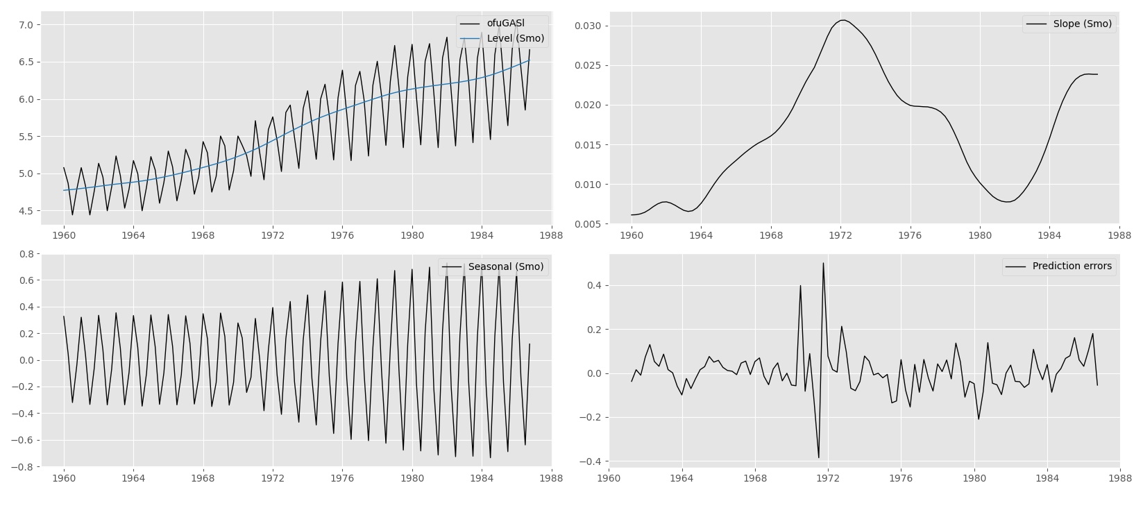
Signal and noise are key concepts in time series analysis and forecasting. The signal in a time series represents the information of interest for the analyst. We aim to extract the signal as accurately as we can from a time series because the signal facilitates decision-making and forecasting. In general, the signal identifies the structural dynamic dependencies in the time series. These structures lead to the formulation of an optimal forecast function. Noise on the other hand is just... well noise. Noise is what remains from the time series after we have accounted for the signal. The statistical formulation of the signal and the noise in the time series is the most important task for a time series analyst. As the signal usually is subject to different dynamic features, it is often decomposed into different components of interest such as trend, seasonal and cycle. In this approach, we obtain the Structural Time Series Model which is set up in terms of these directly interpretable components.

The next question is: "how do we decompose a time series into signal and noise?". The short answer is "we apply a filter". The more elaborate answer is provided below.

Formulating a statistical model

To find the serial or "dynamic" correlation structure in the time series, we formulate a statistical model. We quote from the seminal work of Professor Harvey, A. (1989): the salient characteristics of a time series are a trend, which represents the long-run movements in the series, and a seasonal pattern which repeats itself after some time. A model of the series will need to capture these characteristics. There are many ways in which such a model may be formulated, but a useful starting point is to assume that the series may be decomposed in the following way:

Observed series = trend + seasonal + irregular

where the 'irregular' component reflects non-systematic movements in the series. The model is an additive one. A multiplicative form,

Observed series = trend x seasonal x irregular

may often be more appropriate. However, a multiplicative model may be handled within the additive framework by the simple expedient of taking logarithms.
The advantage of an explicit statistical model is not only that it makes the underlying assumptions clear but that, if properly formulated, it has the flexibility to represent adequately the movements in time series which may have widely differing properties. Hence it is likely to yield a better description of the series and its components. The other motive underlying the construction of a univariate time series model is the prediction of future observations. As a rule, the model used for description should also be used as the basis for forecasting, and the fact that a sensible description of the series is an aim of model-building acts as a discipline for selecting models which are likely to be successful at forecasting.

Structural time series models

The Structural Time Series Model allows the explicit modelling of the trend, seasonal and error term, together with other relevant components for a time series at hand. It aims to present the stylised facts of a time series in terms of its different dynamic features which are represented as unobserved components. In the book of Harvey, A. (1989) it is stated as follows: The statistical formulation of the trend component in a structural model needs to be flexible enough to allow it to respond to general changes in the direction of the series. A trend is not seen as a deterministic function of time about which the series is constrained to move for ever more. In a similar way the seasonal component must be flexible enough to respond to changes in the seasonal pattern. A structural time series model therefore needs to be set up in such a way that its components are stochastic; in other words, they are regarded as being driven by random disturbances. A framework that is flexible enough to handle the above requirements is the State Space model.
The unobserved components can be extracted with the use of filters. More specifically, Time Series Lab adopts the celebrated Kalman filter which is widely seen as a highly effective tool for analysing time series in fields such as economics, finance, engineering, medicine, and many more.

State Space models and the Kalman filter

For an extensive discussion of State Space Models and its accompanying Kalman filter we refer to the books of Harvey (1989) and Durbin and Koopman (2012).
The aim of the State Space Model is to provide a unifying specification of linear time series models. The central part of the model is the state vector that contains all relevant dynamic features of the time series. The state vector evolves over time by means of a linear dynamic system of equations. For example, consider the picture below for a state vector that contains trend (with level and slope, or "growth") and seasonal components.

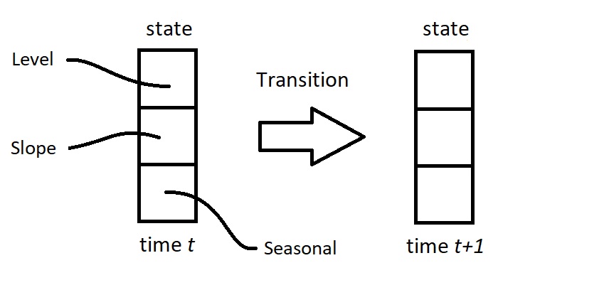
The next step is to establish the optimal move from the state at time $t$ to the one at time $t+1$. For example, in the case of daily data, assume that time $t$ occurs on a Monday. Based on historical data, we have determined the trend and seasonal effects for this Monday. Hence, we have an estimate of the signal (trend plus seasonal) available for time $t$. When the data point for this Monday has been observed, we can establish how close the estimated signal has been. We can measure the prediction error as a result. The next challenge is to determine an estimate (or a prediction) of the seasonal effect for the next day, which is then for a Tuesday. It makes sense to adjust the earlier estimate for Tuesday based on the most recent prediction error, although the error is for a Monday. But how to make this adjustment? How to weight the current estimate and the prediction error of the day before? Here the Kalman filter comes in to play: it provides the optimal weights for this updating step, or for this transition step from Monday to Tuesday (and next, from Tuesday to Wednesday, etc.).
The State Space Model is a very powerful tool which opens the way for the handling of a wide range of time series models. Once a model has been put in state space form, the Kalman filter can be applied straightforwardly. It also opens up other estimation algorithms for prediction, filtering, smoothing, and forecasting. It also solves issues related to missing entries in the time series.
The essence of the Kalman filter is summarised by Harvey, A. (1989) as follows: The Kalman filter rests on the assumption that the disturbances and initial state vector are Normally distributed. A standard result on the multivariate Normal distribution is then used to show how it is possible to calculate recursively the distribution of the state, conditional on the information set at time t, for all t from 1 to the end of the time series. These conditional distributions are themselves Normal and hence are completely specified by their means and covariance matrices. It is these quantities which the Kalman filter computes. It can be shown that the mean of the conditional distribution of the state is an optimal estimator of the state, in the sense that it minimises the mean square error (MSE). When the Normality assumption is dropped, there is no longer any guarantee that the Kalman filter will give the conditional mean of the state vector. However, it is still an optimal estimator in the sense that it minimises the mean square error within the class of all linear estimators.

Linear estimator

We can conclude that the Kalman filter produces optimal estimates of the signal and its components for a class of linear time series models, including the Structural Time Series Model. So what if we need a non-linear estimator? We encounter these situations in for example volatility modelling or the modelling of count data (number of goals scored by a football team, number of earthquakes in a region, or number of Covid-19 cases to name a few), but many more situations can arise. Time Series Lab offers a powerful alternative for non-linear time series modelling and the methodology that is developed for this class of estimators is described in the next article.

Bibliography

Durbin, J. and Koopman, S. J. (2012). Time series analysis by state space methods. Oxford university press.
Harvey, A. (1989). Forecasting, Structural Time Series Models and the Kalman Filter. Cambridge: Cambridge University Press. doi:10.1017/CBO9781107049994