Time Series Lab
Advanced Time Series Forecasting Software

Preface
Time Series Lab is a platform that facilitates the analysis, modelling, and forecasting of time series in a highly interactive way with much graphical support. The users can base their analyses on a large selection of time series approaches, including Box-Jenkins models, exponential smoothing methods, score-driven location models and basic structural time series models. Therefore, users only concentrate on selecting models that fit the data best.Furthermore, Time Series Lab allows the users to select a wide range of dynamic components that are related to, for example, trend, seasonal and stationary cycle processes, in order to build their own time series models. Time Series Lab fully relies on advanced state space methods such as the Kalman filter and related smoothing algorithms. These methods have proven to be very effective in providing powerful solutions for many time series applications. For example, Time Series Lab can handle missing values in all model settings.
The software is developed by R. Lit (Nlitn) and Prof. S.J. Koopman in cooperation with Prof. A.C. Harvey. Copyright © 2019-2025 Nlitn.
How to cite Time Series Lab:
We recommend citing the software as follows, depending on your preferred format:
APA
Lit, R., Koopman, S. J., & Harvey, A. C. (2025). Time Series Lab (Version 3.0.0) [Computer software]. https://timeserieslab.comBibTeX
@misc{lit2025tsl,
  author       = {Rutger Lit and S. J. Koopman and A. C. Harvey},
  title        = {Time Series Lab},
  year         = {2025},
  version      = {3.0.0},
  howpublished = {\url{https://timeserieslab.com}},
  note         = {Computer software}
}MLA
Lit, Rutger, et al. Time Series Lab. Version 3.0.0, 2025, https://timeserieslab.com.Chicago
Lit, Rutger, S. J. Koopman, and A. C. Harvey. Time Series Lab. Version 3.0.0. 2025. https://timeserieslab.com.
Feedback: we appreciate your feedback on the program. Please let us know by sending an email to feedback@timeserieslab.com.
Bugs: encountered a bug? Please let us know by sending an email to bugs@timeserieslab.com.
Contact: or questions about Time Series Lab or inquiries about commercial versions of the program, please send an email to info@timeserieslab.com.
See this section for known issues with the software.
Manual
Contents
1 Getting started
1.1 Installing and starting TSL
1.2 Frontpage
1.3 Time Series Lab modules
2 Connect to database
2.1 Select database connection
2.1.1 Search in database
2.1.2 Download series
3 Select & prepare data
3.1 Database
3.1.1 Load database
3.1.2 Save database
3.1.3 Time axis specification
3.1.4 Select dependent variable
3.1.5 Data transformation
3.2 Graphical inspection of the data
3.2.1 Type of plots
3.2.2 Plot area
3.2.2.1 Data characteristics and statistical tests
3.2.2.2 Undocking the plot area
4 Pre-built models
4.1 Model selection
4.2 Score-driven models
4.2.1 Auto detect optimum p, q
4.3 Model averaging
4.3.1 Equal weights averaging
4.3.2 Least squares
4.3.3 Restricted least squares
4.3.4 Forecast variance weighted
5 Build your own model
5.1 Structural time series models
5.1.1 Level
5.1.2 Slope
5.1.3 Seasonal short
5.1.4 Seasonal medium
5.1.5 Seasonal long
5.1.6 Cycle short / medium / long
5.1.7 ARMA(p,q) I and II
5.1.8 Explanatory variables
5.1.8.1 Select variables
5.1.8.2 Lag finder
5.1.8.3 Settings
5.1.9 Intervention variables
6 Estimation
6.1 Edit and fix parameter values
6.2 Estimation options
7 Graphics and diagnostics
7.1 Selecting plot components
7.2 Plot area
7.3 Additional options
7.3.1 Plot confidence bounds
7.3.2 Add lines to database
7.3.3 Select model / time series
7.3.4 Plot options
7.4 Print diagnostics
7.4.1 State vector analysis
7.4.2 Missing observation estimates
7.4.3 Print recent state values
7.4.4 Print parameter information
7.4.5 Residual summary statistics
7.4.6 Residual diagnostics
7.4.7 Outlier and break diagnostics
7.4.8 Model fit
7.5 Save components
8 Forecasting
8.1 Forecast components
8.2 Additional options
8.2.1 Plot confidence bounds
8.2.2 Select model / time series
8.2.3 Plot options
8.3 Load future
8.4 Save forecast
8.5 Output forecast
9 Text output
10 Model comparison
10.1 Loss calculation procedure
10.2 Start loss calculation
11 Batch module
A Dynamic models
B State Space models
C Score-driven models
D Submodels of score-driven models
D.1 The ARMA model
D.2 The GARCH model
Bibliography
Getting started
If you’re interested in time series analysis and forecasting, this is the right place to be. The Time Series Lab (TSL) software platform makes time series analysis available to anyone with a basic knowledge of statistics. Future versions will remove the need for a basic knowledge altogether by providing fully automated forecasting systems. The platform is designed and developed in a way such that results can be obtained quickly and verified easily. At the same time, many advanced time series and forecasting operations are available for the experts.
There are a few key things to know about TSL before you start. First, TSL operates using a
number of different steps. Each step covers a different part of the modelling process. Before you can
access certain steps, information must be provided to the program. This can be, for example, the
loading of data or the selection of the dependent variable. The program warns you if information is
missing and guides you to the part of the program where the information is missing. We will discuss
each step of the modelling process and use example data sets to illustrate the program’s
functionality.
Throughout this manual, alert buttons like the one on the left will provide you with important
information about TSL.
Furthermore, throughout the software, info buttons, like this blue one on the left, are positioned
where additional information might be helpful. The info button displays its text by hovering the
mouse over it.
TSL uses its algorithms to extract time-varying components from the data. In its simplest form, this is just a Random walk but it can be much more elaborate with combinations of Autoregressive components, multiple Seasonal components, and Explanatory variables. You will see examples of time-varying components throughout this manual. The workings and features of TSL are discussed in Chapter 3–11. If you are more interested in Case studies and see TSL in action, go to Chapter 12.
We refer to Appendix A – D for background and details of time series methodology. Appendix A illustrates the strength of dynamic models and why dynamic models are often better in forecasting than static (constant over time) models. Several of the algorithms of Time Series Lab are based on State Space methodology, see Harvey (1990) and Durbin and Koopman (2012) and the score-driven methodology, see Creal et al. (2013) and Harvey (2013). Appendix B discusses the mathematical framework of state space models and Appendix C discusses the mathematical framework of score-driven models. Knowledge of the methodology is not required to use TSL but is provided for the interested reader. Appendix D shows that well-known models like ARMA and GARCH models are submodels of score-driven models.
1.1 Installing and starting TSL
Time Series Lab comes in two versions, the Home edition and the Enterprise edition. The Home edition can be downloaded for free from https://timeserieslab.com. It has almost every feature and algorithm that the Enterprise edition has. The main difference is that the Home edition is restricted to univariate time series analysis. The commercial Enterprise edition supports companies and institutions to process large volumes of time series in a sequential manner. It further allows TSL to be modified and extended on an individual basis. Also, additional modules can be added to TSL, creating a hands-on platform that is finely tuned towards the particular needs of the user(s). More information can be obtained by sending an email message to info@timeserieslab.com.
Windows 10 64bit and Windows 11 64bit are the supported platforms. TSL can be started by double-clicking the icon on the desktop or by clicking the Windows Start button and selecting TSL from the list of installed programs. TSL is generally light-weight under normal circumstances. It needs less than 600 MB hard-disk space and 600 MB RAM.
1.2 Frontpage
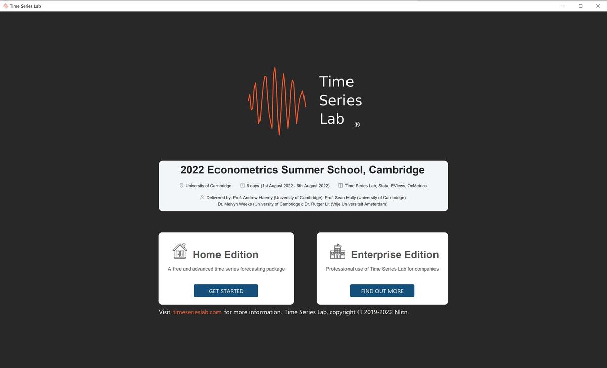
After starting the Home edition of TSL, you see the screen as shown in Figure 1.1. It shows TSL’s logo at the top of the page. The information banner in the middle of the screen displays relevant updates on Time Series Lab. Examples are, information on upcoming new versions of TSL or organized courses / summer schools / winter schools which involves TSL in any way. Information is refreshed every eight seconds and currently does not hold any sponsored content.
The Get Started button leads you to the Database page where you can load your data set. The Find out more buttons opens the web browser and shows information of the TSL Enterprise edition.
Within TSL, you can always return to the Front page by clicking File ▸ Front page in the menu bar at the top of the page.
Front page of TSL Home edition
1.3 Time Series Lab modules
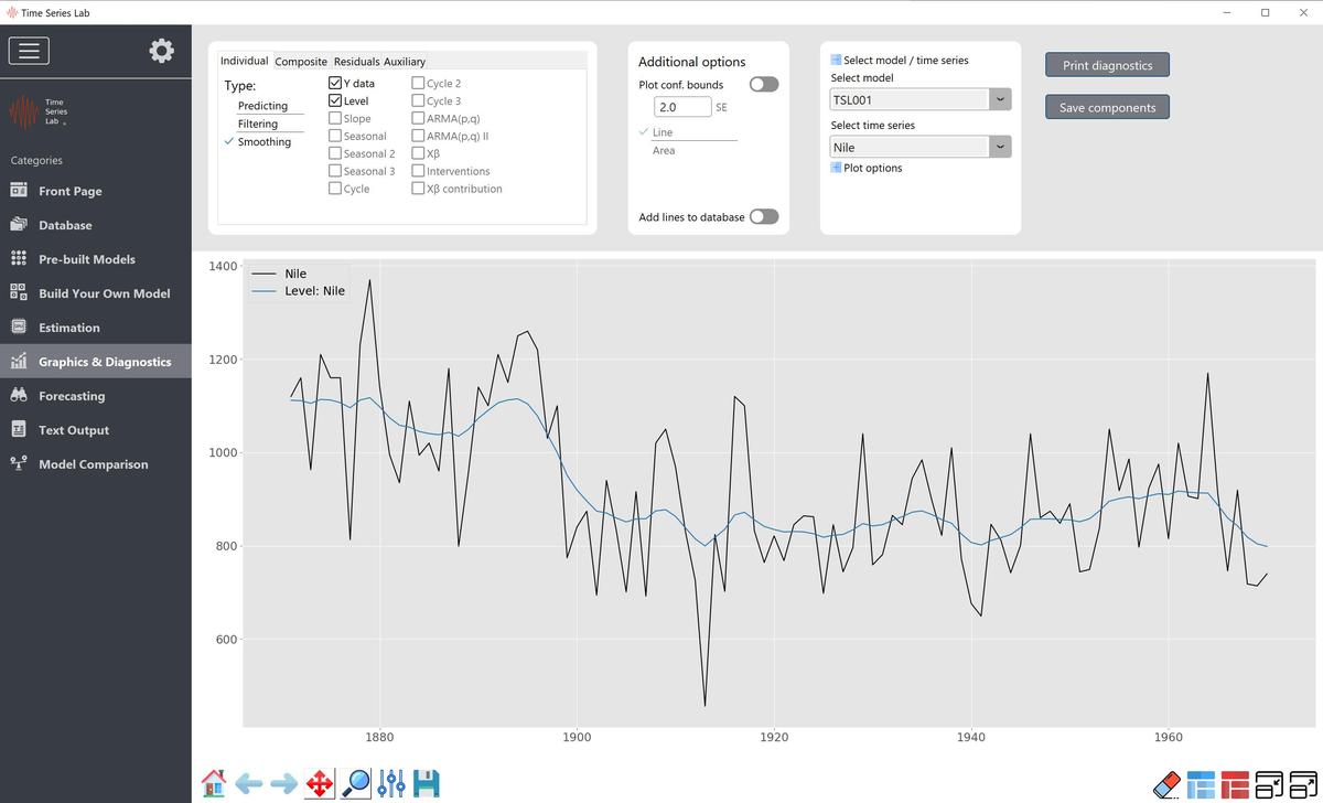
The modules of TSL can be accessed by clicking the buttons located at the left of the screen, see Figure 1.2. The modules are:
- Connect to Database
- Select & Prepare data
- Pre-built models
- Build Your Own Model
- Estimation
- Graphics & Diagnostics
- Forecasting
- Text Output
- Model Comparison
- Batch Module
All modules are described in detail in the following chapters. The Batch module allows you to program and schedule TSL yourself without going through all the menus and pages manually.
Modules of TSL are accessed by the buttons on the left of the screen
Connect to database
There are currently two ways of getting data in TSL. The first method is with a database connection to an API server and this method is discussed in this chapter. The second method is by manually loading a data file. This option is discussed in Chapter 3. To connect to a database via an API server, navigate to the Connect to Database page.
2.1 Select database connection
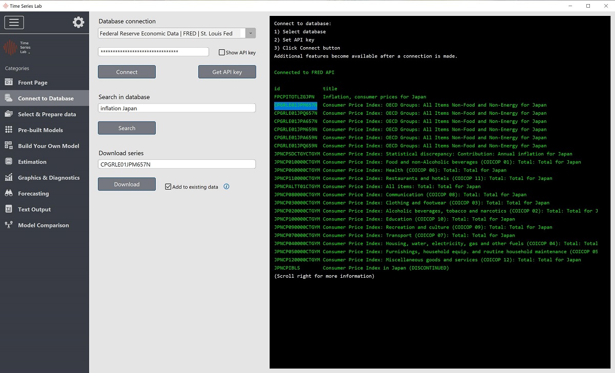
Currently the only available database connection is to the Federal Reserve Economic Data — FRED — St. Louis Fed database. We will add more connections in the future. Let us know if you have suggestions! To connect to a database, perform the following steps:
- 1.
- Select a database from the drop-down menu
- 2.
- Set the API key
- 3.
- Click the connect button
If you do not have an API key to the selected database, you can request one by clicking the Get API key button which will lead you to a sign-up page to request an API key. After a successful connection is made, additional features become available.
2.1.1 Search in database
The search in database option allows you to search for keywords in the database you are connected to. For example, in Figure 2.1 we searched for inflation Japan and the search results from the API server are displayed in the right side of the screen. You might need to scroll down and/or to the right to see all information that was received from the API server.
Connect to database page
2.1.2 Download series
A time series can be downloaded by providing the series ID to the Download series entry field. The simplest way of setting the ID is by double clicking the ID in the text field (right side screen). Alternatively, you can manually type the ID or highlight the ID in the text field and click the right-mouse key followed by clicking Select for download.
Tick the checkbox Add to existing data if you want TSL to add the newly downloaded data to the existing database of previously downloaded series. Note that downloaded data can be added to the existing database only if the frequency matches (quarterly, monthly, etc.). If not, the current database is overwritten with the most recent downloaded data.
Press the Download button to download the series and if this is succesfull, the time series is placed in the TSL database and you are brought to the Select & Prepare data page for further processing.
Select & prepare data
The first step in any time series analysis is the inspection and preparation of data. In TSL, clicking the button as shown on the left brings you to the data inspection and preparation page, see also Figure 3.1. You are also directed to this page after clicking the Get Started button on the Front page. The Nile data set that comes bundled with the installation file of TSL is used as illustration.
3.1 Database
3.1.1 Load database
The data set is loaded and selected from the file system by pressing the Load database button or by clicking File ▸ Load data.
Important: The data set should be in column format with headers. The format of the data should
be *.xls(x), or *.csv, *.txt with commas as field separation. The program (purposely) does not sort
the data which means that the data should be in the correct time series order before loading it into
the program.
Data inspection and preparation page
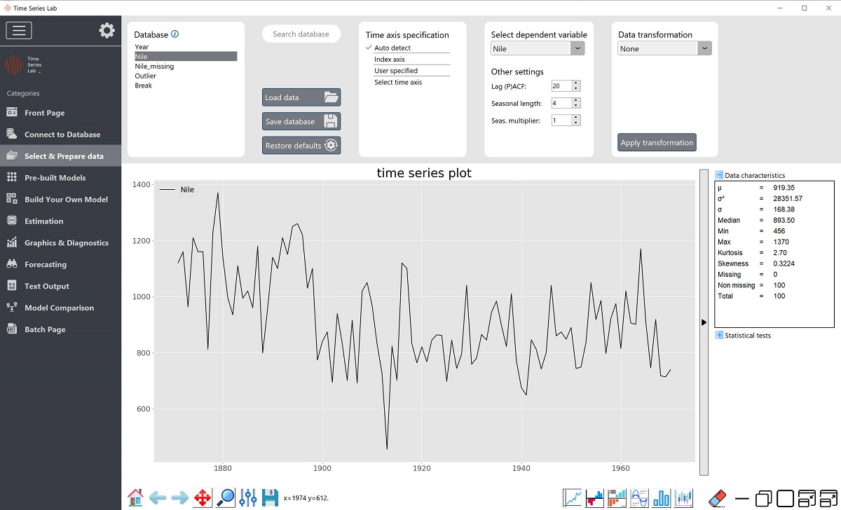
After loading the data, the headers of the data columns appear in the Database section at the top
left of the page. TSL automatically plots the second column of the database after loading. Plot a
different variable by clicking on another header name. Ctrl-click or Shift-click to plot multiple
variables in one graph. As shown in 3.1, the Nile data is currently highlighted and plotted.
3.1.2 Save database
The loaded data set can also be saved to the file system. This will not be useful right after loading but extracted signals from the modelling process are added to the Database at a later stage and can therefore be easily saved for further processing. Additionally, transformed variables, see Section 3.1.5, appear in the Database section as well.
3.1.3 Time axis specification
For time series analysis, time is obviously an important factor. As mentioned in Section 3.1.1, the loaded database should already be in the correct time series order before loading it in TSL. A time series axis can be specified as follows. First, TSL tries to auto detect the time axis specification (e.g. annual data, daily data) from the first column of the data set. In the case of the Nile data illustration in Figure 3.1, it finds an annual time axis specification. If the auto detection fails, the program selects the Index axis option which is just a number for each observation, $1, 2, 3, \ldots$.
You can specify the time axis manually as well via the User specified option or the Select time
axis option. The User specified option, opens a new window in which the user can specify the
date and time stamp of the first observation and the interval and frequency of the time
series. The newly specified time axis shows up in the plot after pressing confirm (and
exit). The Select time axis option allows the user to select the time axis from the loaded
database. If the time axis format is not automatically found by the program the user
can specify this via the Format input field. The text behind the info button ![]() tells
us:
tells
us:
Specify date format codes according to the 1989 C-standard convention, for example:
2020-01-27: %Y-%m-%d
2020(12): %Y(%m)
2020/01/27 09:51:43: %Y/%m/%d %H:%M:%S
Specify ‘Auto’ for auto detection of the date format.
Note that a time axis is not strictly necessary for the program to run and an Index axis will always
do.
3.1.4 Select dependent variable
The so-called y-variable of the time series equation is the time series variable of interest, i.e. the time series variable you want to model, analyze, and forecast. You can specify the dependent variable by selecting it from the drop-down menu located under the Select dependent variable section of the Database page. Alternatively, the dependent variable is automatically selected if a variable is selected to be plotted by clicking on it. In our example, the highlighted variable Nile also appears in the Select dependent variable drop down menu. The dependent variable needs to be specified because without it, the software cannot estimate a model.
3.1.5 Data transformation
If needed, you can transform the data before modelling. For example if the time series consists of
values of the Dow Jones Index, a series of percentage returns can be obtained by selecting
percentage change from the Data transformation drop-down menu followed by clicking the Apply
transformation button. Note that the (original) variable before transformation should
be highlighted before applying the transformation to tell the program which variable
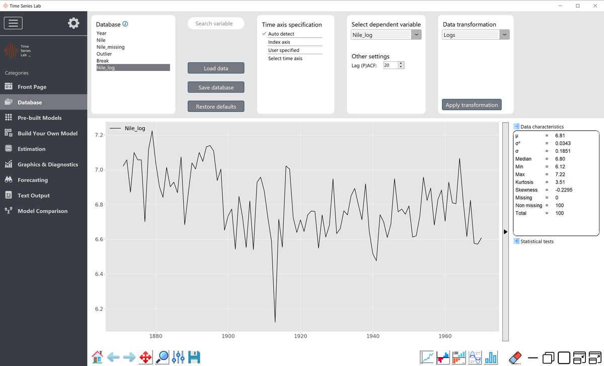
to transform. An example is given in Figure 3.2 where the Nile data is transformed by
taking logs. The newly transformed log variable (Nile_log) is added to the variables in the
Database section and is automatically highlighted and plotted after the transformation.
Transformations can be combined by applying transformations to already transformed
variables. Newly created transformed variables can be removed from the database by right
mouse clicking the variable and selecting the Delete from database option from the popup
menu.
Depending on the selection, spin boxes under the Apply transformation button become visible to
provide additional input.
Lag operator:
Lagged variables can be added to the model as well. Often these are explanatory variables, e.g. $X_{t-1}$. Lagging a time series means shifting it in time. The number of periods shifted can be
controlled by the Add lag spin box which becomes visible after selecting the Lag operator from the
menu. Note the text behind the information button ![]() that says:
that says:
Please note that values > 0 are lags and values < 0 are leads
Lag all operator:
Same as Lag operator but all lags in between are added to the database as well.
Differencing:
A non-stationary time series can be made stationary by differencing. For example, if $y_t$ denotes the value of the time series at
period $t$, then the first difference of $y_t$ at period $t$ is equal to $y_t - y_{t-1}$, that is, we subtract the observation at time $t-1$ from the observation at time $t$. TSL accommodates for this
procedure since differencing is common practice among time series researchers. However, the
methodology of TSL allows the user to explicitly model non-stationary time series and
differencing is not strictly necessary. Note the text behind the information button ![]() that tells
us:
that tells
us:
Time Series Lab allows the user to explicitly model non-stationary components like trend and seasonal. However,
users might prefer to make the time series stationary by taking first / seasonal differences before modelling.
Please note that missing values are added to the beginning of the sample to keep the time series length equal to the
original time series length before the difference operation.
Scaling:
Estimating a time series that consist of several very small or large values could potentially lead to
numerical instabilities. This can be resolved by scaling the time series to more manageable numbers.
For example, if sales data is in euros and numbers are high, the time series could be
scaled down to model sales in millions, for example. Alternatively sales in Logs can be
modelled.
Truncate:
After selecting Truncate, two spinboxes appear which allows you to specify the lower and upper
bound. These values are in the same units as the time series is in and set all observations outside of
the bounds to missing values. Note that missing values can easily be taken into account by
TSL.
Winsorize:
After selecting Winsorize, two spinboxes appear that allows you to specify the lower and upper
percentage bound. All observations outside of the percentage bounds are set to the values
corresponding to the lower and upper percentages. This means that, in contrast to Truncate, they
are not set to missing values.
Data inspection and preparation page: Logs of Nile data
3.2 Graphical inspection of the data
3.2.1 Type of plots
Different types of time series plots can be activated by selecting one of the six plot types at the bottom right of the Database page.
- Time series: this just plots the selected time series.
- Autocorrelation function (ACF): this describes how well the value of the time series at time $t$ is related with its past values $t-1,t-2,\ldots$. This plot (in combination with the PACF plot) is often used to determine the $p$ and $q$ values in ARIMA models. The lags of the (P)ACF plot can be controlled by the spinbox below Other settings.
- Partial autocorrelation function (PACF): this describes how well the value of the time series at time $t$ is related with a past value with the correlation of the other lags removed. For example, it takes into account the correlation between the values at time $t$ and time $t-2$ without the effect of $t-1$ on $t$. This plot (in combination with the ACF plot) is often used to determine the $p$ and $q$ values in ARIMA models.
- Spectral density: the spectral density and the autocovariance function contain the same information, but expressed in different ways. Spectral analysis is a technique that allows us to discover underlying periodicities for example to find the period of cycle components in the times series. The periodicity of the signal is 2.0 / value on the x-axis.
- Histogram plot: this plots the selected time series in histogram format.
- Seasonal subseries: this plots the seasons from a time series into a subseries, e.g. time series of only Mondays, followed by only Tuesdays, etc. For example if your data is hourly data, set the Seasonal length spinbox to 24 and the Seas. multiplier to 1 to obtain a plot of the intraday pattern. To obtain a plot of the weekdays, set the Seasonal length spinbox to 24 and the Seas. multiplier to 7.
3.2.2 Plot area
The plot area can be controlled by the buttons on the bottom left of the Database page. The pan/zoom, zoom to rectangle, and save figure are the most frequently used buttons.
- Home button: reset original view.
- Left arrow: back to previous view.
- Right arrow: forward to next view.
- Pan/zoom: left mouse button pans (moves view of the graph), right button zooms in and out.
- Zoom to rectangle: this zooms in on the graph, based on the rectangle you select with the left mouse button.
- Configure subplots: this allows you to change the white space to the left, right, top, and bottom of the figure.
- Save the figure: save figure to file system (plot area only). To make a screenshot of the complete TSL window, press Ctrl-p.
Right mouse click on the graph area, opens a popup window in which you can select to set the Titles of the graph, the time-axis, add or remove the legend, and add or remove the grid of the plot area.
3.2.2.1 Data characteristics and statistical tests
When clicked, the vertical arrow bar on the right of the screen shows additional information about the selected time series. The Data characteristics panel shows characteristics of the selected time series. It shows statistics like mean, variance, min, and maximum value, among others characteristics. It also shows the number of missing values in the time series. It should be emphasized that:
Missing values can easily be taken into account in TSL. Even at the beginning of the time series.
The Statistical tests panel shows the result of the Augmented Dickey-Fuller test and KPSS test. The null hypothesis of the Augmented Dickey-Fuller test is: \[ H_0: \text{a unit root is present in the time series} \] If the p-value is $<$ 0.05, $H_0$ is rejected. For our example Nile dataset, we have a p-value of 0.0005 so we reject the null hypothesis. The null hypothesis of the KPSS test is: \[ H_0: \text{the series is stationary} \] If the p-value is $<$ 0.05, $H_0$ is rejected. For our example Nile dataset, we have a p-value of $< 0.01$ so we reject the null hypothesis. The results of both test may look contradicting at first but it is possible for a time series to be non-stationary, yet have no unit root and be trend-stationary. It is always better to apply both tests, so that it can be ensured that the series is truly stationary. Possible outcomes of applying these stationary tests are as follows:
- Case 1: Both tests conclude that the series is not stationary - the series is not stationary
- Case 2: Both tests conclude that the series is stationary - the series is stationary
- Case 3: KPSS indicates stationarity and ADF indicates non-stationarity - the series is trend stationary. Trend needs to be removed to make series strict stationary. The detrended series is checked for stationarity.
- Case 4: KPSS indicates non-stationarity and ADF indicates stationarity - the series is difference stationary. Differencing is to be used to make series stationary. The differenced series is checked for stationarity.
See also this link for more information. We emphasize that in TSL there is no need to make a series trend or difference stationary but you can if you prefer. One of the many advantages of TSL is that trends and other non-stationary components can be included in the model.
3.2.2.2 Undocking the plot area
The plot area can be undocked from the main window by clicking the undock draw window in the bottom right of the screen. Undocking can be useful to have the graph area on a different screen but most of its purpose comes from the area underneath the plot area. For the Enterprise edition of TSL, this area is used to select and summarize all selected time series. Since the Home edition of TSL is for univariate time series analysis only, this area is just blank and serves no further purpose.
Pre-built models
After loading our time series data in TSL, it is time to analyze the time series and extract
information from it. The fastest way to extract information from your time series is by using the
Pre-built models page. Select the models you want to use, set the training and validation sample,
click the green arrow which says Process Dashboard and let TSL do the rest. But which time series
model to use?4.1 Model selection
TSL comes with a range of pre-programmed time series models for you to choose from, all with its
own characteristics and features. An overview of the available models in TSL is given in Table 4.1.
This table provides a short description of the models and, for the interested reader, references to the
scientific journals the models were published in. You can select one or multiple models and TSL will
give you results of all the selected models in one go. The alternative is to construct your own time
series model based on the selection of components. This option will be discussed in Chapter 5.
If you are not sure which time series model to select, use the following guideline. Does your time series data exhibit a trend or seasonal pattern? If neither is present in the time series, start with Exponential Smoothing or the Local Level model. If your data does contain trending behavior, use the Holt-Winters or the Local Linear Trend model. If your time series shows a seasonal pattern as well, use the Seasonal Holt-Winters or the Basic Structural model. The last two models and the Local Level + Seasonal model take seasonal effects into account, something which can greatly improve model fit and forecast accuracy. To set the Seasonal period length (s), enter a number in one of the Spinboxes located beneath one of the seasonal models. Note that the seasonal period needs to be an integer (whole number). Fractional seasonal periods can be used when you build your own model, see Chapter 5. TSL tries to determine the seasonal period from the loaded data and pre-enters it. If it cannot find the seasonal period length, it reverts to the default period length of 4. You can of course always change this number yourself. Typical examples of seasonal specifications are:
- Monthly data, s=12
- Quarterly data, s=4
- Daily data, s=7 (for day-of-week pattern)
Once the models are selected, set the length of the training sample by dragging the slider or by pressing
one of the buttons of the pre-set training and validation sample sizes. Model parameters are
optimized based on the data in the training sample and the rest of the data belongs to the
validation sample which is used to assess out-of-sample forecast accuracy. As a rule of thumb, a
model is preferred over a rival model, if model fit in the training sample (e.g. in-sample RMSE) is
better (lower) AND out-of-sample forecast accuracy in the training sample is better as
well. The latter is often harder to achieve compared to improving the fit in the training
sample.
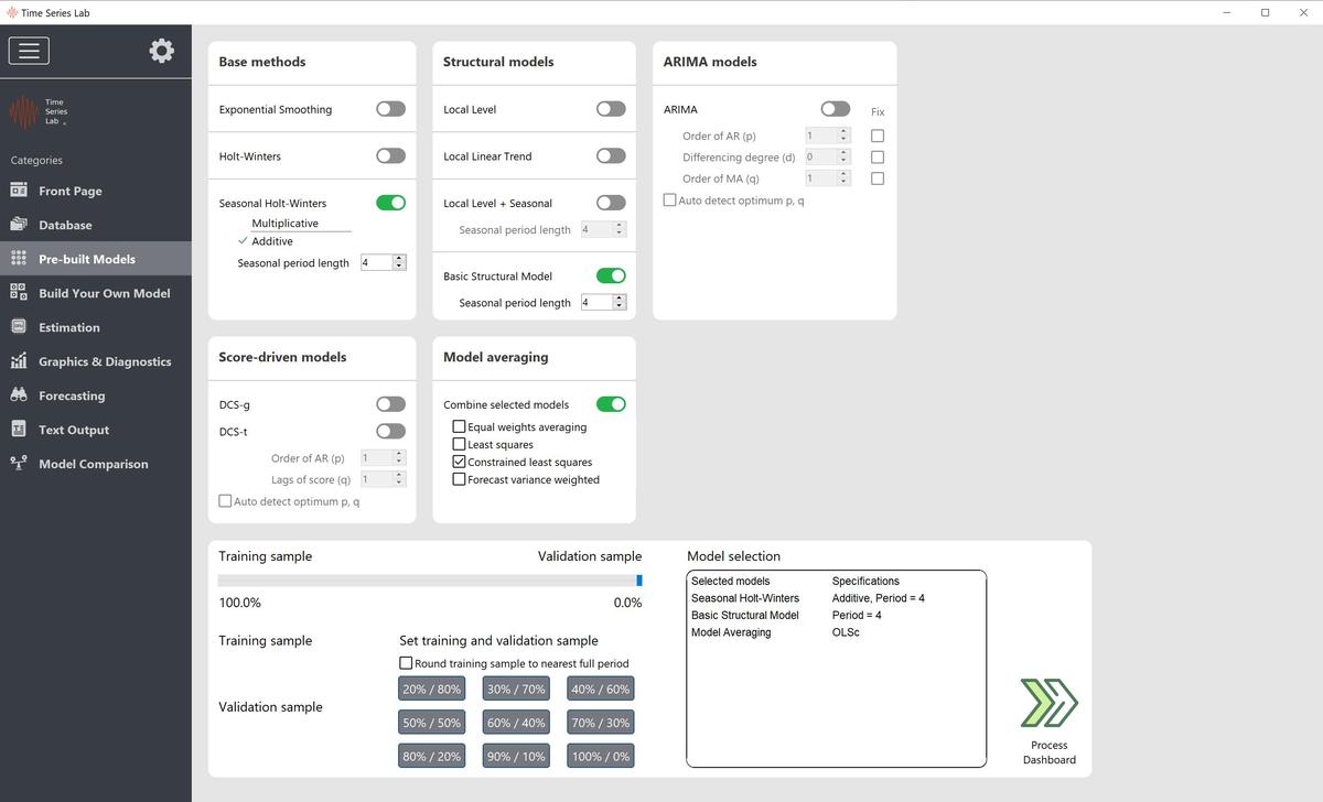
The ENERGY dataset that comes bundled with TSL has quarterly data on energy consumption. It’s an old dataset but good for illustrative purposes since energy consumption changes with the four seasons. If we would like to model the ENERGY dataset with a Seasonal Holt-Winters model with Additive seasonality (period = 4), a Basic Structural Model (period = 4), and we want to combine the forecasts of both models by Constrained Least Squares Model Averaging, we set TSL as shown in Figure 4.1
Models of TSL and references to scientific literature
The table reports the models of TSL with features and reference to the literature.
| Model description | Model features | Reference |
| Base models |
|
|
| Exponential Smoothing Holt-Winters Seasonal Holt-Winters | Forecasts produced using exponential smoothing methods are weighted averages of past observations, with the weights decaying exponentially as the observations get older. In other words, the more recent the observation the higher the associated weight. This framework generates reliable forecasts quickly and for a wide range of time series, which is a great advantage and of major importance to applications in industry, see https://otexts.com. | |
| Structural models |
|
|
| Local Level Local Linear Trend Local Level + Seasonal Basic Structural Model | By structural time series models we mean models in which the observations are made up of trend, seasonal, cycle and regression components plus error. In this approach it is assumed that the development over time of the system under study is determined by an unobserved series of vectors α1,…,αn, with which are associated a series of observations y1,…,yn; the relation between the αt’s and the yt’s is specified by the state space model. In TSL, complex dynamics like multiple seasonalities can modelled with state space models, more information is presented in Chapter 5. Many time series models are special cases of the state space model. | Durbin and Koopman (2012), Harvey (1990) |
| ARIMA models |
|
|
| ARIMA(p,d,q) | As with structural time series models, ARIMA models typically regard a univariate time series yt as made up of trend, seasonal and irregular components. However, instead of modelling the various components separately, the idea is to eliminate the trend and seasonal by differencing at the outset of the analysis. The resulting differenced series are treated as a stationary time series. ARIMA is an acronym for AutoRegressive Integrated Moving Average and any ARIMA model can be put into state space form. | |
| Score-driven models |
|
|
| DCS-g, DCS-t | Score-driven models are a class of linear and non-linear models that can be used to analyse and forecast a wide range of time series. Score-driven models are so versatile that well-known models like ARMA and GARCH models are subclasses of score-driven models, see Appendix D, Appendix C, and Chapter 4.2 for more information. | Creal et al. (2013), Harvey (2013) |
| Model averaging |
|
|
| Equal weights averaging Least Squares Restricted Least Squares Forecast Variance Weighted | The idea of combining forecasts from different models as a simple and effective way to obtain improvements in forecast accuracy was introduced by Bates and Granger (1969). In almost all cases we cannot identify the true data generating process of the time series, and combining different models can play a complementary role in approximating it. | Bates and Granger (1969), Timmermann (2006), Hansen (2008) |
Model settings of TSL on the Pre-built models page
4.2 Score-driven models
Many time series models are build on the assumption of Normally distributed errors. Despite its popularity, many time series require a different distribution than the Normal distribution. One of the major advantages of score-driven models is that you are not restricted to the Normal distribution, in fact you can choose almost any probability distribution. In many cases, using a different probability distribution than the Normal leads to increases in model fit and out-of-sample forecast accuracy.
Score-driven models are a class of linear and non-linear models that can be used to analyse and forecast a wide range of time series. Score-driven models are so versatile that well-known models like ARMA and GARCH models, are subclasses of score-driven models, see also Appendix D. Furthermore, the score-driven model encompasses other well-known models like the autoregressive conditional duration (ACD) model, autoregressive conditional intensity (ACI) model, and Poisson count models with time-varying mean. We refer to Appendix C, Creal et al. (2013), and Harvey (2013) for more information on score-driven models.
The Time Series Lab project started with the Time Series Lab - Dynamic Score Edition which focused solely on score-driven models and had many probability distributions that the user could choose from. At the time of writing of this manual, the Time Series Lab - Dynamic Score Edition is still available for downloaded but the idea is to merge all Time Series Lab projects into one time series package. That would mean that all score-driven models with their specific distributions and features will, over time, be available in the main Time Series Lab package. A start with the merging of score-driven models into the current package is made by introducing the Normal score-driven model (DCS-g) and the Student t score-driven model (DCS-t). The Student t distribution has, so called, fatter tails compared to the Normal distribution. Fatter tails mean that outliers have a higher probability of occuring. The benefit of using the Student t distribution is shown in Case study 12.5.
4.2.1 Auto detect optimum p, q
Both the ARIMA and score-driven models can easily be extended with additional lag structures. This can be done by setting the p and q parameters. For ARIMA models, there is the extra option of setting the parameter d which allows for the series to be differenced before being modelled to make the time series stationary. We refer to the literature in Table 4.1 for more information on lag structures.
Often, including more lags leads to a higher likelihood value which is a measure of model fit. However, including more lags comes at the price of more model parameters that need to be determined. The optimal number of lags p and q, based on the Akaike Information Criterion (AIC), can be found by selecting the Auto detect optimum p, q option. TSL determines the optimum number of lag structures by applying the Hyndman-Khandakar algorithm, see Hyndman and Khandakar (2008).
4.3 Model averaging
The idea of combining forecasts from different models as a simple and effective way to obtain improvements in forecast accuracy was introduced by Bates and Granger (1969). In almost all cases we cannot identify the true Data Generating Process of the time series, and combining different models can play a role in approximating it. A popular way to combine the individual predictions is to consider the following linear model: \begin{equation}\label{eq:mdl_avg} Y_t = X_t^{'} \beta + \varepsilon_t, \qquad t = 1, \ldots, T \end{equation} where $\varepsilon_t$ is white noise which is assumed to have a normal distribution with zero mean and unknown variance, $Y_t$ is our observed time series, and $X_{i,t}$ the point forecast from one of our selected models for $i = 1, \ldots, k$ with $k$ the number of selected models and $T$ the length of our time series. The parameter vector $\beta$ can be chosen in different ways each leading to a different combination of models.
4.3.1 Equal weights averaging
This is the simplest of the model averaging techniques. All weights are chosen equal, meaning that each point forecast has weight $1/k$ which gives: \[ \hat{\beta}_{EWA} = (\tfrac{1}{k},\ldots,\tfrac{1}{k}) \qquad \text{and} \qquad \tilde{Y}_t^{EWA} = \tfrac{1}{k} \sum_{i=1}^k X_{i,t}. \]
4.3.2 Least squares
A natural extension to the Equal weights averaging method is to determine the weights by Least squares estimators. This OLS approach to combine forecasts was proposed by Granger and Ramanathan (1984). They used OLS to estimate the unknown parameters in the linear regression model of (4.1). The OLS estimator of the parameter vector β of the linear regression model is \[ \hat{\beta}_{OLS} = \left( X^{'} X \right)^{-1} X^{'} Y. \] Note that the $T \times (k+1)$ matrix $X$ has an intercept in its first column. The estimate $\hat{\beta}_{OLS}$ is unrestricted meaning that negative weights are allowed. This model often performs very well in the training set but not always for the validation set. To counter this issue of overfitting, Restricted least squares might be a good alternative.
4.3.3 Restricted least squares
For the restricted OLS approach, the unknown parameters in the linear regression model (4.1) are obtained by restricting each of the elements of $\hat{\beta}_{OLSc}$ to lie between 0 and 1. Furthermore, the elements of $\hat{\beta}_{OLSc}$ must sum to 1. Note that the $T \times k$ matrix $X$ does not have an intercept. The estimate $\hat{\beta}_{OLSc}$ is restricted and negative weights cannot occur.
4.3.4 Forecast variance weighted
This method is also called Bates-Granger averaging. The idea is to weight each model by $1/\sigma_i^2$, where $\sigma_i^2$ is its forecast variance. In practice the forecast variance is unknown and needs to be estimated. This leads to \[ \hat{\beta}_{FVW,i} = \frac{1/\hat{\sigma}_i^2}{\sum_{j=1}^k \hat{\sigma}_i^2}, \] where $\hat{\sigma}_i^2$ denotes the forecast variance of model $i$ which we estimate as the sample variance of the forecast error $e_{i,t} = X_{i,t} - Y_t$ within the training sample period.
Build your own model
Instead of selecting a pre-defined model from the Pre-built models page, you can also build your
own model. This requires some basic knowledge and logic but no extensive statistical knowledge is
needed. With the help of this chapter, you can come a long way. If in doubt, you can always try
adding or removing components to see the effect on model fit and forecast performance. TSL is
written in a robust way and adding components should not break anything so you are free to
experiment. If things break, please let us know so we can make TSL even more robust!
5.1 Structural time series models
The Structural Time Series Model allows the explicit modelling of the trend, seasonal and error term, together with other relevant components for a time series at hand. It aims to present the stylised facts of a time series in terms of its different dynamic features which are represented as unobserved components. In the seminal book of Harvey (1990) it is stated as follows: “The statistical formulation of the trend component in a structural model needs to be flexible enough to allow it to respond to general changes in the direction of the series. A trend is not seen as a deterministic function of time about which the series is constrained to move for ever more. In a similar way the seasonal component must be flexible enough to respond to changes in the seasonal pattern. A structural time series model therefore needs to be set up in such a way that its components are stochastic; in other words, they are regarded as being driven by random disturbances.” A framework that is flexible enough to handle the above requirements is the State Space model.
The Basic structural time series model is represented as: \[ y_t = \mu_t + \gamma_t + \varepsilon_t, \qquad t = 1,\ldots,T \] where $y_t$ is our time series observation, $\mu_t$ is the trend component, $\gamma_t$ the seasonal component, and $\varepsilon_t$ the error term, all at time $t$. In TSL you can select other or additional components like cycle ($\psi_t$), autoregressive components (AR$_t$), Explanatory variables ($X_t\beta_x$), and Intervention variables ($Z_t\beta_z$). We discuss each dynamic component and its characteristics.
A summary of all selected components of the Build your own model page and its characteristics
is given in the blue Model specification area of TSL.
Important: Dynamic components each have unique characteristics and can be combined to form
complicated models that reveal hidden dynamics in the time series.
Intermezzo 1: Time-varying components
TSL extracts a signal from the observed time series. The difference between the observed time series and the signal is the noise, or the error. The methodology of TSL relies heavily on filtering time series with the aim to remove the noise from the observation and to secure the signal in the time series and possibly to identify the different components of the signal. We are interested in the signal because it provides us the key information from the past and current observations that is relevant for the next time period. In its simplest form, the signal at time $t$ is equal to its value in $t-1$ plus some innovation. In mathematical form we have \[ \alpha_t = \alpha_{t-1} + \text{some innovation}, \]
with $\alpha_t$ being the signal for $t=1,\ldots,T$ where T is the length of the time series. The innovation part is what drives the signal over time. A more advanced model can be constructed by combining components, for example \[ \alpha_t = \mu_{t} + \gamma_t + X_t\beta, \]
where $\mu_t$ is the level component, $\gamma_t$ is the seasonal component, $X_t\beta$ are explanatory variables, and where each of the components have their own updating function.
5.1.1 Level
The Level component $\mu_t$ is the basis of many models. If only the (time-varying) level is selected the resulting model is called the Local Level model and, informally, it can be seen as the time-varying equivalent of the intercept in the classical linear regression model. The time-varying level uses observations from a window around an observation to optimize model fit locally. How much each observation contributes to the local level fit is optimized by the algorithms of TSL.
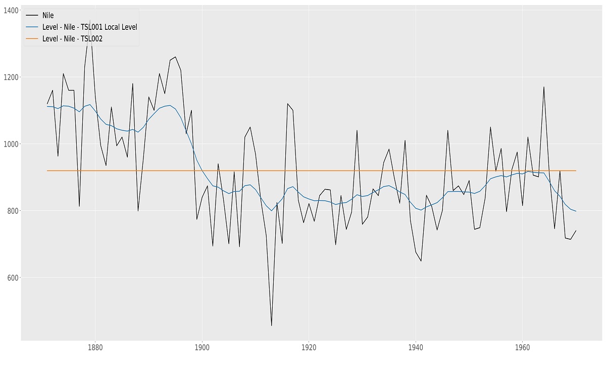
The fixed version of the level is often used in combination with other components. We will see examples of the use of a fixed (or static) level later in this manual. Figure 5.1 shows the result of fitting the local level to the Nile data. For completeness, fixed level is added for comparison. Needless to say, the time-varying local level model fits the data better.
Nile data with Local level model, time-varying and static
5.1.2 Slope
The slope component $\nu_t$ can only be selected in combination with the level component. It is used for time series that exhibits trending behavior. If both a time-varying level and time-varying trend are selected, the model selection corresponds to the Local Linear Trend model. Certain combinations of the level and slope component can have interesting effects on the smoothness of the extracted signal. For example, if the level is set to fixed and the slope to time-varying, often a much smoother signal is obtained. In the literature, the resulting model is known as an Integrated Random Walk model. Varying levels of smoothness can also be achieved by setting the order of the trend to a higher number. In general (but definitely not always), the higher the order, the smoother the resulting signal.
5.1.3 Seasonal short
The inclusion of the Seasonal component γts in our model allows us to model a wide range of time
series. Time series can contain a variety of seasonal effects and in TSL you can add three seasonal
components to your model if needed. The info button
![]() , next to the seasonal short component,
tells us:
, next to the seasonal short component,
tells us:
Seasonal period length is the number of time points after which the seasonal repeats. Examples of seasonal specifications are:
Monthly data, s = 12.
Quarterly data, s = 4.
Daily data, when modelling the weekly pattern, s = 7.
The seasonal period can be a fractional number. For example, with daily data, specify a period of 365.25 for a seasonal that repeats each year, taking leap years into account. See the case studies on the timeserieslab.com website for more information on how to specify seasonals.
Number of factors specifies the seasonal flexibility. Note that a higher number is not always better and parsimonious models often perform better in forecasting.
It’s best to explain the seasonal component with an example. Let’s say our time series is weekly data on gasoline consumption, see also Case study 12.2. With gasoline consumption, fluctuations are to be expected throughout the year due to, for example, temperature changes during the year. For the moment assume we have 52 weeks in a year and we would therefore specify s = 52.0 as the seasonal period. For the number of factors, we specify 10. As a rule of thumb, do not take the maximum amount of factors (which is s/2) because this makes the seasonal very flexible which is good for your training sample fit but often performs worse in forecasting. Another disadvantage of taking a “large” number of factors is that the model becomes slower to estimate. This is however a general guideline and experimenting might be necessary. Future version of TSL determine the optimal set of factors.
Now let’s assume that our data on gasoline consumption is still weekly data but we realize that we need s > 52.0 since we have more than 52.0 weeks in a year. On top of that our dataset also contains a leap year. We therefore set the seasonal period to s = 365.25∕7 = 52.179 where 365.25 is the average number of days in a year in a four year time span including one leap year and 7 the number of days in one week. This small change of 52.179 - 52.0 = 0.179 in seasonal period length can make a big difference in forecasting as we will see in Case study 12.2.
Another example would be hourly electricity demand. We can expect electricity demand to change within a 24h cycle with more energy demand during the daytime and less during night time. For this example we would set s = 24.0 to model the 24h cycle within a day, see also Case study 12.10.
5.1.4 Seasonal medium
If we want to include only one seasonal component in our model we should take the Seasonal short.
But if we want to model a double seasonal pattern we can include Seasonal medium $\gamma_t^m$ as well. Continuing with our hourly electricity demand example, we can use the seasonal
medium to model the day of week pattern on top of the 24h intraday pattern. We can
expect energy demand to be lower during the weekend since, for example, many business
are closed. To model this, we set the seasonal period length of the seasonal medium
component to $s = 7 \times 24 = 168$. For the number of factors, we can specify a number around
20.
Continuing with our hourly electricity demand example, we can use the seasonal long $\gamma_t^l$ to
model the demand pattern throughout the year. Since energy demand often changes
with the four seasons of the year we can $s = 24 \times 365.25 = 8766.0$. Note that our time
series needs to be long and preferably several times s to take the yearly pattern into
account.
A combination of seasonal patterns can strongly increase forecast precision as we will see in Case
study 12.10.
The cycle and seasonal components have similarities since both components have repeating
patterns. The big difference however is that the seasonal component has a fixed, user set, period
while the period of the cycle components $\psi_t^s, \psi_t^m, \psi_t^l$ are determined from the data. This becomes
useful if you want to, for example, model GDP and determine the length of the business cycle. Time
series can contain multiple cycles as we will see in Case study 12.4 where an El Nino time series
contains complex dynamics with three cycle patterns. The statistical specification of a cycle $\psi_t$ is as
follows:
\begin{equation}
\begin{bmatrix}
\psi_t \\
\psi^*_t
\end{bmatrix}
= \rho
\begin{bmatrix}
\text{cos}\, \lambda_c & \text{sin}\, \lambda_c \\
-\text{sin}\, \lambda_c & \text{cos}\, \lambda_c
\end{bmatrix}
\begin{bmatrix}
\psi_{t-1} \\
\psi^*_{t-1}
\end{bmatrix}
+
\begin{bmatrix}
\kappa_{t} \\
\kappa^*_{t}
\end{bmatrix} ,
\qquad t = 1,\ldots,T
\end{equation}
where $\lambda_c$ is the frequency, in radians, in the range $0 < \lambda_c < \pi$, $\kappa_t$ and $\kappa^*_t$ are two
mutually uncorrelated white noise disturbances with zero means and common variance $\sigma_{\kappa}^2$, and $\rho$ is a damping factor with $0 \leq \rho \leq 1$. Note that the period is $2 \pi / \lambda_c$.
The stochastic cycle becomes a first-order autoregressive process if $\lambda_c = 0$ or $\lambda_c = \pi$.
The parameters $\lambda_c, \rho, \sigma_{\kappa}^2$ are determined by the algorithms of TSL.
An autoregressive moving average process of order $p, q$, ARMA(p,q), is one in which the current value is based on the previous $p$ values and error terms occurring contemporaneously and at various times in the past.
It is written as:
\[
x_t = \phi_1 x_{t-1} + \phi_2 x_{t-2} + \ldots + \phi_p x_{t-p} + \theta_1 \epsilon_{t-1} + \theta_2 \epsilon_{t-2} + \ldots + \theta_p \epsilon_{t-p} + \epsilon_t,
\]
with $\epsilon_t$ being white noise, $\phi_1,\ldots,\phi_{t-p}$ being the AR coefficients that determine the persistence of the process, and $\theta_1,\ldots,\theta_{t-p}$ being the MA coefficients.
The process is constrained to be stationary; that is, the AR and MA coefficients are restricted to represent a stationary process.
If this were not the case there would be a risk of them being confounded with the random walk component in the trend. Since the ARMA(p, q) processes of TSL are
stationary by construction, the processes fluctuates around a constant mean which is zero in
our case. The persistence of fluctuations depend on the values of the ϕ parameters.
When there is a high degree of persistence, shocks that occur far back in time would
continue to affect $y_t$, but by a relative smaller amount than shocks from the immediate
past. If an autoregressive process is needed that fluctuates around a number other than
zero, add a fixed (constant) Level component in combination with the autoregressive
process.
A second ARMA(p, q) process can be added to the model. In this setup, the first autoregressive
process captures persistent and long run behavior while the second autoregressive process captures
short term fluctuations.
Explanatory variables play an important and interesting role in time series analysis. Adding
explanatory variables can significantly improve model fit and forecasting performance of your model.
The difficulty often lies in finding explanatory variables that significantly contribute to model fit and
forecasting performance. If we switch Explanatory variables on, a new window opens like the one
presented in Figure 5.2. Alternatively, if the window does not popup, you can click the Adjust
selection button to bring the window to the front. You can choose between Manually
and Automatically. Manually means, all selected variables will be added to the model,
automatically means, variables are selected based on a significance level that you can set, see
also Section 5.1.8.3. In Automatic mode, a TSL algorithm adds and removes variables
and iteratively re-estimates the model in between to end up with a set of explanatory
variables that all have their t-stats above a specified threshold. We note that our algorithm
does not simply remove variables one-by-one. Variables can re-enter the equation at
later stages to increase the probability of ending up with an optimal set of explanatory
variables. Important: We are fully aware that people engage in heated debates on do or do not
remove explanatory variables based on statistical relevance. We do not contribute to
that debate here, you just have the option to auto-remove variables or leave them all in.
In the explanatory variables window you see a list of all variables in the database with
colored indicators in front of them. Hovering with the mouse over the info button To select multiple explanatory variables, click the first variable, then Ctrl-click the next variable, and so on. Click
on a variable and press Ctrl-a to select all variables. A consecutive range of variables can be included by clicking the
first variable and Shift-click the last variable in the range.
The color in the first column indicates how likely it is that the variable contributes significantly to the overall
model fit. The green variables should be considered first and the red ones last. The Indicator lights are based on a
pre-analysis and only when the full dynamic model is estimated can we say something about the actual contribution
of the variable.
Important: The explanation of the indicators is in the bottom right corner of the newly opened window. The
colors show the likelihood that an explanatory variable contributes significantly to the fit of the
model. The more significant a variable is, the higher it is on the color ranking scale. Of course, we
can only be certain after we estimate the model but it gives an idea. The colors are determined
based on a regression of the currently selected time series on the rest of the variables in the
database, as in
\begin{equation}\label{eq:vV}
v_t = V_t\beta + \epsilon_t, \qquad t = 1,\ldots,T,
\end{equation}
where $v$ and $V$ correspond to $y$ and $X$ with dynamics removed.
The idea is to use information from the last model to remove dynamics (trend, seasonal, etc.) from the $y$ and $X$ data to end up with $v$ and $V$.
After that, a regression from $v$ on $V$ should now reveal relationships that cannot be explained by dynamics alone and could therefore explained by the regression variables.
The more significant $\hat{\beta}_i$ is, the higher the corresponding regression variable $X_i$ will be on the color ranking scale.
Some variables are not allowed in the model. These are variables that have values that cannot be
represented by a number, like the values in the date column for example.
The black dot indicator deserves a bit more attention. It is possible to add a black indicator
variable to the model. However, it should be used with a lot of caution. The reason is as follows:
black indicator variables are time series that are added to the database after estimation.
Typically, these are extracted signals like level or seasonal. Take the following basic structural
model
\begin{equation}\label{eq:bsm_xvar1}
y_t = \mu_t + \gamma_t + \varepsilon_t, \qquad t = 1,\ldots,T
\end{equation}
with level $\mu_t$ seasonal $\gamma_t$ and irregular $\varepsilon_t$.
When this model is estimated in TSL (Chapter 6 explains Estimation), the extracted components $\mu_t$ and $\gamma_t$ can be added to the database and show up in the explanatory variables window where they get a black indicator. If now the following model is
estimated:
\begin{equation}\label{eq:bsm_xvar2}
y_t = \mu_t + X_t \beta + \varepsilon_t, \qquad t = 1,\ldots,T
\end{equation}
where $X_t$ is the black indicator (Smoothed) seasonal component that was obtained from model
(5.3) we could think we have the same model as in 5.3. However, this is not true and we
introduced two errors in the model. The first one is that each component in a state space
model has its own variance (we discuss error bounds in Chapter 7.3.1) but if extracted
dynamic components are added to the model as explanatory variables, the variance gets
deflated and does not represent the true uncertainty in the extracted signals anymore.
The second problem is that the smoothed seasonal is based on all data so adding that
to a new model for the same time series $y_t$ is using more observations than you would
normally do for prediction. You will see that you artificially increase model fit by doing
this.
A reason to still include a black indicator variable is if an extracted signal is used as explanatory
variable in a model with a different time series $y_t$.
The Lag finder module uses the same auxiliary regression as in (5.2) but instead of the
contemporaneous X variables in the dataset, it aims to find candidates for significant lags of the X variables. In time series analysis, often one series leads another. For example, an explanatory
variables at time $t-3$ can explain part of the variation in $y_t$. Instead of trying out all possible lags
of all variables, the lag finder module aims at finding these lags for you. Just as with the regression
of (5.2), we can only be certain if a lagged variable contributes significantly to the model fit after
we estimate the model.
Select the X variable(s) for which you want to find significant lags and press the Lag finder
button. If significant lags are found, they show up with a green indicator light in the explanatory
variable list.
The second tab of the Explanatory variables window is the Settings tab. On this tab we set the
t-stat after which an indicator becomes green on the Select variables tab. We can also set the
Maximum allowed p-value which determines how strict we are in removing variables from the
model in the Automatic removal of explanatory variables. Furthermore, you can set which
method to use to replace missing values in explanatory variables and which method to use
to forecast explanatory variables.
Intervention variables are a special kind of explanatory variables. There are two types, Outliers and
Structural breaks, both are very useful for anomaly detection. For example, early warning systems
rely on anomaly detection, also called outlier and break detection. Could a catastrophic event have
been seen in advance? Take for example sensor readings from an important piece of heavy
machinery. The breaking down of this machine would cost a company a lot of money. If anomalies
were detected in the sensor reading, preventive maintenance might have saved the company from a
break-down of the machine.
For example, if we have the following stochastic trend plus error model
\[
y_t = \mu_t + \lambda Z_t + \varepsilon_t, \qquad t = 1,\ldots,T
\]
where $Z_t$ is an intervention (dummy) variable and $\lambda$ is its coefficient.
If an unusual event is to be treated as an outlier, it may be captured by a pulse dummy variable at time $t = \tau$, that is
\begin{equation}
Z_t =
\begin{cases}
0 & \text{for } t \neq \tau \\
1 & \text{for } t = \tau .
\end{cases}
\end{equation}
A structural break in the level at time $t$ may be modelled by a level shift dummy,
\begin{equation}
Z_t =
\begin{cases}
0 & \text{for } t < \tau \\
1 & \text{for } t \geq \tau .
\end{cases}
\end{equation}
If we switch Intervention variables on, a new window opens. Alternatively, if the window does not
open, you can click the Adjust selection button to bring the window to the front. Just as with
explanatory variables, you can choose between Manually and Automatically. If set to manual, the
window opens up showing the Select interventions tab. Here you can specify time points where you
want to position outliers and / or structural breaks. Hovering with the mouse over the info button
Select outliers and structural breaks. If an Outlier and Structural break are set at the same time point, the
Outlier gets precedence.
Add an outlier or structural break by clicking one of the buttons and change the index to reflect
the desired date.
If Automatically is selected, the Settings tab is shown. In the automatic case, TSL finds the
outliers and structural breaks for you. The Lowerbound t-stats and Stop algorithm when both have
to do with the stopping condition of the algorithm. Furthermore, the checkboxes allow you to
exclude outliers or structural breaks from the algorithm. We will see an example of automatic outlier
detection in Case study 12.3, among other.
The Estimation page of TSL looks like Figure 6.1. Getting results from TSL can be
achieved in two ways. The first one was discussed in Chapter 4 by using the Process
Dashboard button. The second one is by using the Estimate button on the Estimation page.
Before you press this button there are certain things useful to know, so let’s discuss
them.
Components that we have selected on the Build your own model page all have corresponding
parameters that can be set, fixed, and / or estimated. After entering the Estimation page, TSL has
set the parameters to rudimentary starting values based on the sample variance of the
selected time series. These values will later be refined depending on what you tell TSL to
do. Model output results depend strongly on the parameters as listed in the Edit and
fix parameter values section. There are five ways in which you can influence parameter
values.
We can say something, in general, about ordering of the five ways based on which setting
obtains results fastest. If we rank the methods in order of speed starting with the fastest method we
have, (4) – (5) – (2, 3) – (1). Starting values can have a big impact on the speed of estimation,
therefore we cannot say if (2) is faster than (3) or vice versa. We are often interested in the best model fit for the validation sample. For this we choose method (1), which is the
default.
The software checks the user input in the Value entry boxes because some parameters are
restricted to a certain range, see for an example Figure 6.2.
The model parameters, also called hyper parameters, can be estimated by Maximum Likelihood with
the BFGS algorithm or No estimation can be selected so that text and graphical output will be
based on the provided starting values. For the majority of the models, maximizing the likelihood is a
routine affair. Note however, that for more complicated models and the increase of the number of
hyper parameters, optimization can be complex. The info button next to the BFGS option tell us
that:
The BFGS method falls in the category of quasi-Newton optimizers. This class of optimizers is applicable to
many optimization problems and is often used to maximize a likelihood function.
Please be aware that finding a global optimum is not guaranteed and trying different starting values increases the
chance of finding the global optimum.
We are not restricted to estimating the full sample in our data set. If needed, we can restrict the
estimation to a smaller sample by setting the Estimation starts at t and Estimation ends at t entry
boxes.
During estimation results can be communicated to you via the Text output page (see also
Chapter 9). You can choose the amount of detail that is communicated by TSL, we
have
Furthermore, we have three buttons under Additional options. The Set default estimates button,
sets the values in the value column back to the rudimentary starting values that were initially there.
The Set default estimates button, sets the values in the value column to the most recent optimized
parameter values.
After the successful estimation of a model, a (hyper) parameter report can be generated.
Clicking the Parameter report button brings us to the Text output page where the parameter report
will be printed. Important: The time it takes to generate the parameter report depends strongly on the number of
hyper parameters, the number of model components, and the length of the time series. The generation of a parameter report can take the amount of time it takes to maximize the likelihood. Plotting components is very simple: it only requires ticking the check box corresponding to the
component you would like to see in the graph. Note that some components are greyed out as they
were not selected as part of the model. We have four plot tabs in the upper left corner of the
program,
The difference between Predicting, Filtering and Smoothing is further explained in
Appendix B. These three options are available for State Space models which is every
model combination on the Build your own model page and the Local Level, Local Linear
Trend, Local Level + Seasonal, and Basic Structural Model on the Pre-built models
page.
The majority of the buttons below the plot area is explained in Chapter 3 except two new buttons.
These are the add subplot and remove subplot button. Just as the name says, they add and
remove subplots from the plot area. The plot area of TSL can consist of a maximum of
nine subplots. Subplots can be convenient to graphically summarize model results in one
single plot with multiple subplots. Notice that after clicking the add subplot button an
empty subplot is added to the existing graph which corresponds to no check boxes being
ticked. Important: The components that are graphically represented in a subplot directly correspond to the
check boxes that are ticked. Clicking on a subplot activates the current plot settings.
Notice that by clicking a subplot, a blue border appears shortly around the subplot as a
sign that the subplot is active. If you hover the Clear all button, the tooltip window
shows:
The Clear all button clears everything from the figure including all subplots. To have more refined control over
the subplots, right-mouse click on a subplot for more options.
If you hover the Add subplot button, the tooltip window shows:
Click on a subplot to activate it. Notice that by clicking on a subplot, the checkboxes in the top left of the
window change state based on the current selection of lines in the subplot.
If not all checkbox settings correspond with the lines in the subplot, switch the tabs to show the rest of the
selection.
Several more plot options are available on the Graphics page. We discuss them here.
You have the option to include confidence bounds in the plot. The methodology that is used if you
Build your own model is based on the State Space model, see also Appendix B. One advantage of
the state space framework is that the statistical properties of the state, which holds all components,
is fully known at each time $t$. This in contrast to many other time series models that do not possess
this property. We can therefore include confidence bounds for all models that are based on State
Space models. To add confidence bounds, first switch Plot conf. bounds on, and then select
the component you want to plot. If plots are requested for other types of models, the
Plot conf. bounds option is not available. The width of the confidence interval can be
controlled by changing the number in the SE field. Furthermore, you can choose the
Line option, which plots two extra lines corresponding to the bounds of the confidence
interval, or select Area to give the whole confidence area a shaded color, see also Figure
7.3.
This option is switched off by default. If switched on, every following line that is plotted is added to
the database of the Database page, see also Chapter 3. This allows you to quickly store extracted
signals combined with the data you originally loaded. Use the Save database button on the
Database page to store your data, see also Section 3.1.2.
The drop-down menu corresponding to Select model collects all the previously estimated models.
This is a powerful feature since you can now compare extracted signals from different models in the
same plot. This feature becomes even more powerful in comparing forecast abilities of different
models, see Chapter 10. There are a couple of important things you should know because under
some circumstances models cannot be compared and the drop-down menu is reset to only the most
recent model. This happens if you:
In all other cases, the drop-down menu will grow with every new model you estimate.
The drop-down menu corresponding to Select time series holds all time series that were
estimated with the model currently selected by the Select model drop-down menu. For the
TSL Home edition you will see only one time series at a time.
Plot options gives you control over the line transformation, line type, and line color of the
lines you want to plot. The defaults are, line transformation: None, line type: Solid, and
line color: Default color cycle. The latter means that for every line drawn a new color is
chosen according to a pre-set color order. You can always choose a color yourself from the
drop-down menu or by clicking the color circle to the right of the Line color drop-down
menu.
Clicking the Print diagnostics button in the top right corner of the Graph page opens the window
as shown in Figure 7.4. We are presented the option to chose a model, a time series,
and a selection of diagnostics, and additional output. Note that not all models have the
same number of diagnostic options. Some of the options are reserved for State Space
models only since they have confidence bounds at their disposal (see Section 7.3.1) which
some tests are based on. All output of the diagnostic tests is printed to the Text output
page.
Select this option for a statistical analysis of the components of the state vector at time $t_2$ (last
time point of training sample). TSL prints the name of the component, the value at time $t_2$, the
standard error, the t-stat (value / standard error), and the probability corresponding to the
t-stat.
If your time series contains missing values, select this option to give estimates for the missing
values. The estimates are printed to the Text output page. If you want to store these
values, save the Smoothed estimates via the Save components option, see also Section
7.5.
Select this option to print the last X values of the state for the selected components and for
Predicting, Filtering, and Smoothing. X is the number of recent periods which you can
specify.
Select this option to print the values of the optimized parameters. For State Space models, a
column with q-values is added which are the ratios of the variance parameters. A 1.0 corresponds to
the largest variance in the model.
Select this option to print residual characteristics of the standardized residuals. TSL prints Sample
size, Mean, Variance, Median, Minimum, Maximum, Skewness, and Kurtosis. For State Space
models, additional residuals are available, these are Smoothed residuals and Level residuals
which are used for Outlier and Break detection, see also Chapter 5.1.9 and Case study
12.3.
Depending on the model specification, residuals can be assumed to come from a Normal
distribution. This is for example the case with State Space models. Due to the Normal assumption,
residuals can be formally tested to come from a Normal distribution. Several tests are available.
There are tests that target specific parts of the Normal distribution like Skewness and Kurtosis and
there are tests that combine both, for example the Jarque-Bera test. Other tests like Shapiro-Wilk
and D’Agostino’s K2 take a different approach. TSL provides Statistics and Probabilities
for each of them. In general, a Probability $< 0.05$ is considered a rejection of the null
hypothesis:
\[
H_0: \text{Standardized residuals are Normally distributed}.
\]
Furthermore, a Serial correlation test is provided to test for residual autocorrelation based on the
Ljung-Box test. Currently the number of lags are chosen by TSL. In future versions, the
lags can be set by the user. TSL provides the Lags it tested, the Test statistic, and the
corresponding Probability. In general, a Probability $< 0.05$ is considered a rejection of the null
hypothesis:
\[
H_0: \text{Standardized residuals are independently distributed}.
\]
Outlier and Break detection, see also Chapter 5.1.9 and Case study 12.3 is based on Auxiliary
residuals, see Durbin and Koopman (2012) p59. Outliers and breaks above a provided threshold can
be printed to screen.
Model fit is printed to the Text output page after each model estimation. This output can also be
printed by selecting the Model fit option.
All components from the Individual, Composite, Residuals, and Auxiliary tabs on the Graph page
can be saved to the file system. Click the Save components button in the upper right corner of the
Graph page. Select the components you want to save or click the Select all components button to
select all components, followed by Save selected.
The available components to forecast are a subset of the components that can be plotted on the
Graphics page with one exception, Y forecast. For all models, Total signal and Y forecast are
exactly equal, except for their confidence intervals. Note that confidence intervals are only available
for State Space models. The difference between confidence intervals for Total signal and Y forecast
has to do with the extra error term that State Space models possess, see Appendix B for more
background. As a result, confidence intervals for Y forecast are wider than for Total
signal.
You can choose between one-step-ahead forecasting and multi-step-ahead forecasting.
The difference is how many steps we forecast ahead standing at the end of the Training
sample (time point $t_2$). For one-step-ahead forecasting, we make a forecast one step
ahead, update the data and go to the next time point ($t_2+1$) and the forecasting process
repeats. For multi-step-ahead forecasting, we stay at time $t_2$ and forecast 1-step, 2-step,
3-step,$\ldots$,n-step-ahead. If the Validation sample has size 0, meaning the Training sample is
100% of your data, one-step-ahead forecasting and multi-step-ahead forecasting are the
same.
For the Local Level model, the multi-step-ahead forecasts form a straight line because we cannot
update our model anymore with new data, see also Figure 8.2. For models with, for
example, seasonal components, multi-step-ahead forecasts are no longer straight lines since
these models have dynamics regardless if new data comes in. We see examples of this in
Chapter 12.
The difference between the observations in the Training sample and the forecasts can be
quantified into a loss function. If Y forecast or Total signal are selected, three loss functions are
added to the right side of the plot area. The loss functions are Root Mean Squared Error (RMSE),
Mean Absolute Error (MAE), and Mean Absolute Percentage Error (MAPE). A more substantial
evaluation of Forecasting performance is provided on the Model comparison page, see also
Chapter 10.
Some more plot options are available on the Forecast page. We discuss them here.
See Section 7.3.1
See Section 7.3.3
Click the spinboxes to expand or contract the part of the Training and Validation sample that is
displayed on screen. For line colors see Section 7.3.4.
The load future option is for users who have knowledge about the future that they want to
incorporate in the model forecasts. This is mainly used for explanatory variables but can be used for
the y variable as well. If you make multi-step-ahead forecasts and explanatory variables are included
in the model, the explanatory variables need to be forecasted as well. This is the case, for example,
on the model comparison page where forecasts are made up to 50 steps ahead. TSL forecasts the
explanatory variables with the method selected as described in Section 5.1.8.3. If you do not want
TSL to forecast the explanatory variables you can specify them yourselves by loading a dataset with
the load future option. Important: The loaded future data is matches with the main data set by means of comparing
column names. Only if column names of the loaded future data matches the ones (can also be a
subset of the column names) in the main data set, is the future data taken into account.
See Section 7.5
See Section 7.5
Just like plot areas, the Text output are can be undocked with the buttons in the bottom right
of the screen. This way the text area can be placed outside of the main TSL window on for example
a different monitor.
Important: The Model comparison button is only visible if you provided a Validation sample. If you
would have chosen to use all data for the Training sample ($t_2=T$), loss calculations cannot be
made since forecasts cannot be compared with actual values in the Validation sample.
We compare models based on several Loss functions, for example, the Root Mean Squared Error
(RMSE). For the RMSE we have
\begin{equation}\label{eq:rmse}
\text{RMSE}_h = \sqrt{\frac{1}{p-h+1} \sum_{t=t_2}^{t_2+p-h} (y_{t+h} - \hat{y}_{t+h|t})^2},
\end{equation}
with $p$ the length of the Validation sample, $t_2$ the length of the Training sample, $h$ the length of the forecast horizon, and $\hat{y}_{t+h|t}$ the forecast for observation $y_{t+h}$ given the information up to time $t$.
Assume we estimated a model for a time series with length $T=400$ and we took a ratio of $80\%/20\%$ for Training and Validation sample.
This means we have a Training sample with length $t_2 = 320$.
By repeatedly making 1-step-ahead, 2-step-ahead, $\ldots \ldots$, 50-step-ahead forecasts, according
to Equation (10.1), we make a total of 80 $\times$ 1-step-ahead forecasts, 79 $\times$ 2-step-ahead forecasts, 78 $\times$ 3-step-ahead forecasts, $\ldots \ldots$, 31 $\times$ 50-step-ahead forecasts. By obtaining many
forecasts we have a robust way of comparing models with each other based on forecasting performance.
Select the model and time series from the drop-down menus for which you want to calculate
forecast losses. Click the Start loss calculation button in the top right corner of the screen to start
the calculation. When the loss calculation is finished, the selected model shows up in the User
defined models section in the top left of the screen. Select the newly appeared check box and the
corresponding losses appear in the plot area for the loss functions selected under Loss functions.
Repeat the procedure for other models and/or compare the results with losses from the Naive
forecast methods.
Finally, print the selected model loss combinations to the Text output page by clicking the Print model
comparison button.
Why do we need dynamic models? Short answer, many real-world processess are dynamic /
time-varying. The more we can capture dynamics, the better we understand the processes and the
better we can predict them. Many processes exhibit some form of dynamic structure. The list of
examples is endless and contains almost every (academic) field. For example, finance where the
volatility of stock price returns is not constant over time. In Economics, where the sale
of clothing items exhibit strong seasonality due to summer and winter but also daily
seasonal patterns because Saturday will be, in general, a more busy day than Monday,
the trajectory of a rocket in Engineering, The El Niño effect due to change in water
temperature in Climatology, the number of oak processionary caterpillars throughout the
year in Biology, to name a diverse few. If we would be interested in saying anything
meaningful about the examples above we need to deal with time-varyingness in some sort of
way.
We illustrate the strength of dynamic models with figures. The data is the number of
cases of Dengue (logged values) in a region of Venezuela from 2001 to 2017, see Figure
A.1.
Figure A.1 shows the static mean and we can clearly see that a static mean would give a model fit
that can be easily improved on. In the beginning of the sample, the mean is much too high
and during the worst period the static mean is far below the actual number of cases.
Needless to say, we could not use a static model to make accurate forecasts for this
series.
Now consider the situation if we would make the mean time-varying by allowing it to
have some smooth pattern over time. The dynamic mean clearly follows the data much
better.
As it turns out, model fit can be further improved by taking into account the monthly effect of the
time series. The improved model fit is displayed in Figure A.3. The figures in this section can all be
replicated with TSL.
Consider a parametric model for an observed time series $y = \left(y_1',\ldots,y_n' \right)'$ that is formulated conditionally on a latent $m \times 1$ time-varying parameter vector $\alpha_t$, for time index $t=1,\ldots,n$.
We are interested in the statistical behavior of the state vector, $\alpha_t$, given a subset of the data, i.e. the data up to time $t-1$ (forecasting), the data up to time $t$ (filtering) or the whole data set (smoothing).
One possible framework for such an analysis is the state space model, the general form of which is given by
\begin{equation}\label{eq:ssm1}
y_{t}|\alpha_{t} \sim p(y_{t}|\alpha_{t};\psi), \qquad \alpha_{t+1} \sim p(\alpha_{t+1}|\alpha_{t};\psi), \qquad \alpha_1 \sim p(\alpha_1;\psi),
\end{equation}
where $p(y_{t}|\alpha_{t};\psi)$ is the observation density, $p(\alpha_{t+1}|\alpha_{t};\psi)$ is the state transition density with initial density $p(\alpha_1;\psi)$ and $\psi$ is a static parameter vector.
%The state space model in \eqref{eq:ssm1} is a parameter-driven model in the classification of Cox(81).
Minimum mean square error (MMSE) estimates of $\alpha_t$ and MMSE forecasts for $y_t$ can be obtained by the Kalman filter and related smoother methods if the following three conditions are met: (i) the state transition density $p(\alpha_{t+1}|\alpha_{t};\psi)$ for $\alpha_t$ is linear and Gaussian, (ii) the relation between $y_t$ and $\alpha _t$ in $p(y_{t}|\alpha_{t};\psi)$ is linear and (iii) the observation $y_t$ is, conditional on $\alpha_t$, normally distributed.
In other words, $p(y_{t}|\alpha_{t};\psi)$, $p(\alpha_{t+1}|\alpha_{t};\psi)$ and $p(\alpha_1;\psi)$ are Gaussian and the observation and transition relations are linear.
If all three conditions are satisfied, the state space model of \eqref{eq:ssm1} reduces to the linear Gaussian state space model,
\begin{equation}\label{eq:stsm}
\begin{aligned}
y_t &= Z \alpha_t + \varepsilon_t, \qquad & \varepsilon_t &\sim N(0,H_t), & \\
\alpha_{t+1} &=T \alpha_t + \eta_t, \qquad & \eta_t &\sim N(0,Q_t), & \qquad \alpha_1 \sim p(a_1,P_1),
\end{aligned}
\end{equation}
for $t = 1,\ldots,n$ see for example Durbin and Koopman (2012, Part I). The violation of at least one of
the three properties means that the state space model becomes nonlinear and/or non-Gaussian for
which we have to rely on other methods to obtain optimal estimates.
In TSL, we work with Linear Gaussian State Space models and the principle of maximum
likelihood estimation (MLE). The main motivation to use MLE are the well established and well
documented properties of MLE.
Consider a parametric model for an observed time series $y = \left(y_1',\ldots,y_n' \right)'$ that is formulated conditionally on a latent $m \times 1$ time-varying parameter vector $\alpha_t$, for time index $t=1,\ldots,n$.
We are interested in the statistical behavior of $\alpha_t$ given a subset of the data, i.e. the data up to time $t-1$.
One possible framework for such an analysis is the class of score-driven models in which the latent
time-varying parameter vector αt is updated over time using an autoregressive updating
function based on the score of the conditional observation probability density function,
see Creal et al. (2013) and Harvey (2013).
The updating function for $\alpha_t$ is given by
\[
\alpha_{t+1} = \omega + \sum_{i=1} ^p A_i s_{t-i+1} + \sum_{j=1} ^q B_j \alpha_{t-j+1},
\]
where $\omega$ is a vector of constants, $A$ and $B$ are fixed coefficient matrices and $s_t$ is the scaled score function which is the driving force behind the updating equation.
The unknown coefficients $\omega$, $A$ and $B$ depend on the static parameter vector $\psi$.
The definition of $s_t$ is
\[
\qquad s_t = S_t \cdot \nabla_t, \qquad \nabla_t = \frac{\partial \, \log \, p(y_t | \alpha_t, \mathcal{F}_{t-1} ; \psi)}{\partial \alpha_t}, \qquad t = 1,\ldots,n,
\]
where $\nabla_{t}$ is the score vector of the (predictive) density $p(y_t | \alpha_t, \mathcal{F}_{t-1} ; \psi)$ of the observed time series $y = \left(y_1',\ldots,y_n' \right)'$.
The information set $\mathcal{F}_{t-1}$ usually consists of lagged variables of $\alpha_t$ and $y_t$ but can contain exogenous variables as well.
To introduce further flexibility in the model, the score vector $\nabla_{t}$ can be scaled by a matrix $S_t$.
Common choices for $S_t$ are unit scaling, the inverse of the Fisher information matrix, or the square root of the Fisher inverse information matrix.
The latter has the advantage of giving $s_t$ a unit variance since the Fisher information matrix is the variance matrix of the score vector.
In this framework and given past information, the time-varying parameter vector $\alpha_t$ is perfectly predictable one-step-ahead.
The score-driven model has three main advantages: (i) the ‘filtered’ estimates of the
time-varying parameter are optimal in a Kullback-Leibler sense;(ii) since the score-driven models are
observation driven, their likelihood is known in closed-form; and (iii) the forecasting performance of
these models is comparable to their parameter-driven counterparts, see Koopman et al. (2016). The
second point emphasizes that static parameters can be estimated in a straightforward way using
maximum likelihood methods.
Score-driven models encompass several other econometric models, among several well-known like
ARMA models and the GARCH model of Engle (1982). Furthermore the ACD model of Engle and
Russell (1998), the autoregressive conditional multinomial (ACM) model of Russell and
Engle (2005), the GARMA models of Benjamin et al. (2003), and the Poisson count models
discussed by Davis et al. (2005). We now show mathematically how ARMA and GARCH models are
submodels of score-driven models.
Consider the time-varying mean model
\[
y_t = \alpha_t + \varepsilon_t, \qquad \varepsilon_t \sim NID(0, \sigma^2),
\]
for $t = 1,\ldots,T$ and where $NID$ means Normally Independently Distributed. If we apply
the score-driven methodology as discussed in Appendix C and we take p = q = 1 we
have,
\[
\alpha_{t+1} = \omega + \beta \alpha_t + \kappa s_t, \qquad s_t = S_t \cdot \nabla,
\]
where
\[
\nabla_t = \frac{\partial \ell_t}{\partial \alpha_t}, \qquad S_t = -E_{t-1} \left[\frac{\partial^2 \ell_t}{\partial \alpha_t \partial \alpha_t} \right]^{-1},
\]
with
\[
\ell_t = -\frac{1}{2} \, \text{log} \, 2\pi - \frac{1}{2} \, \text{log} \, \sigma^2 - \frac{1}{2\sigma^2}(y_t - \alpha_t)^2.
\]
We obtain
\[
\nabla_t = \frac{1}{\sigma^2}(y_t - \alpha_t), \qquad S_t = \sigma^2,
\]
and $s_t = y_t - \alpha_t$ which is the prediction error.
This means that the score updating becomes
\[
\alpha_{t+1} = \omega + \beta \alpha_t + \kappa (y_t - \alpha_t),
\]
and if we now replace $\alpha_t = y_t - \varepsilon_t$, we have
\[
y_{t+1} = \omega + \beta y_t + \varepsilon_{t+1} + (\kappa - \beta) \varepsilon_t,
\]
and hence score updating implies the ARMA(1,1) model for $y_t$
\[
y_{t} = \omega + \phi y_{t-1} + \varepsilon_{t} + \theta \varepsilon_{t-1},
\]
where $\phi \equiv \beta$ and $\theta = \kappa - \beta$.
Furthermore, if we set $\kappa = \beta$, we obtain the AR(1) model and if we set $\beta = 0$ we obtain the MA(1) model. The above is valid for higher lag orders p, q as well which means that the score-driven framework encompasses the ARMA(p,q) model.
The strong results of the above section holds, with a couple of small changes, for the time-varying variance model as well. Consider the time-varying variance model
\[
y_t = \mu + \varepsilon_t, \qquad \varepsilon_t \sim NID(0, \alpha_t),
\]
for $t = 1,\ldots,T$ and where $NID$ means Normally Independently Distributed. After setting $\mu = 0$ we have the predictive logdensity
\[
\ell_t = -\frac{1}{2} \, \text{log} \, 2\pi - \frac{1}{2} \, \text{log} \, \alpha_t - \frac{y_t^2}{2 \alpha_t}.
\]
We obtain
\[
\nabla_t = \frac{1}{2 \alpha_t^2}y_t^2 - \frac{1}{2 \alpha_t} = \frac{1}{2 \alpha_t^2} (y_t^2 - \alpha_t).
\]
Furthermore we have $S_t = 2 \alpha_t^2$ and we obtain $s_t = y_t^2 - \alpha_t$.
This means that the score updating becomes
\[
\alpha_{t+1} = \omega + \beta \alpha_t + \kappa (y_t^2 - \alpha_t),
\]
and hence score updating implies the GARCH(1,1) model
\[
\alpha_{t+1} = \omega + \phi \alpha_t + \kappa^* y_t^2,
\]
where $\phi = \beta - \kappa$ and $\kappa^* \equiv \kappa$.
Furthermore, if we set $\kappa = \beta$, we obtain the ARCH(1) model. The above is valid for higher lag orders of p, q as well which means that the score-driven framework encompasses the GARCH(p,q) model.
It should be emphasized that a score-driven time-varying variance model with Student $t$ distributed errors is not equal to a GARCH-$t$ model.
Bamston, A. G., M. Chelliah, and S. B. Goldenberg (1997). Documentation of a highly
enso-related sst region in the equatorial pacific: Research note. Atmosphere-ocean 35(3),
367–383.
Bates, J. M. and C. W. Granger (1969). The combination of forecasts. Journal of the
Operational Research Society 20(4), 451–468.
Benjamin, M. A., R. A. Rigby, and D. M. Stasinopoulos (2003). Generalized
autoregressive moving average models. Journal of the American Statistical
association 98(461), 214–223.
Box, G. E., G. M. Jenkins, G. C. Reinsel, and G. M. Ljung (2015). Time series analysis:
forecasting and control. John Wiley & Sons.
Brown, R. G. (1959). Statistical forecasting for inventory control. McGraw/Hill.
Creal, D. D., S. J. Koopman, and A. Lucas (2013). Generalized autoregressive score
models with applications. Journal of Applied Econometrics 28(5), 777–795.
Davis, R. A., W. T. Dunsmuir, and S. B. Streett (2005). Maximum likelihood estimation
for an observation driven model for poisson counts. Methodology and Computing in Applied
Probability 7(2), 149–159.
De Livera, A. M., R. J. Hyndman, and R. D. Snyder (2011). Forecasting time series with
complex seasonal patterns using exponential smoothing. Journal of the American statistical
association 106(496), 1513–1527.
Durbin, J. and S. J. Koopman (2012). Time Series Analysis by State Space Methods (2nd
ed.). Oxford: Oxford University Press.
Engle, R. F. (1982). Autoregressive conditional heteroscedasticity with estimates of the
variance of united kingdom inflation. Econometrica 50(4), 987–1007.
Engle, R. F. and J. R. Russell (1998). Autoregressive conditional duration: a new model
for irregularly spaced transaction data. Econometrica 66(5), 1127–1162.
Granger, C. W. and R. Ramanathan (1984). Improved methods of combining forecasts.
Journal of forecasting 3(2), 197–204.
Hansen, B. E. (2008). Least-squares forecast averaging. Journal of Econometrics 146(2),
342–350.
Harvey, A. C. (1990). Forecasting, structural time series models and the Kalman filter.
Cambridge university press.
Harvey, A. C. (2013). Dynamic Models for Volatility and Heavy Tails: With Applications to
Financial and Economic Time Series, Volume 52. Cambridge: Cambridge University Press.
Harvey, A. C. and S. J. Koopman (1992). Diagnostic checking of unobserved-components
time series models. Journal of Business & Economic Statistics 10(4), 377–389.
Holt, C. C. (2004). Forecasting seasonals and trends by exponentially weighted moving
averages. International journal of forecasting 20(1), 5–10.
Hyndman, R. J. and Y. Khandakar (2008). Automatic time series forecasting: the forecast
package for r. Journal of statistical software 27, 1–22.
Koopman, S. J., A. Lucas, and M. Scharth (2016). Predicting time-varying parameters
with parameter-driven and observation-driven models. Review of Economics and
Statistics 98(1), 97–110.
Li, M., S. J. Koopman, R. Lit, and D. Petrova (2020). Long-term forecasting of el niño
events via dynamic factor simulations. Journal of Econometrics 214(1), 46–66.
Petrova, D., S. J. Koopman, J. Ballester, and X. Rodó (2017). Improving the long-lead
predictability of el niño using a novel forecasting scheme based on a dynamic components
model. Climate Dynamics 48(3), 1249–1276.
Russell, J. R. and R. F. Engle (2005). A discrete-state continuous-time model of financial
transactions prices and times: The autoregressive conditional multinomial–autoregressive
conditional duration model. Journal of Business & Economic Statistics 23(2), 166–180.
Timmermann, A. (2006). Forecast combinations. Handbook of economic forecasting 1,
135–196.
Winters, P. R. (1960). Forecasting sales by exponentially weighted moving averages.
Management science 6(3), 324–342.
5.1.5 Seasonal long
5.1.6 Cycle short / medium / long
5.1.7 ARMA(p,q) I and II
5.1.8 Explanatory variables
![]()
5.1.8.1 Select variables
![]() , you
see
, you
see
The pre-analysis is determined based on results from the last model run.
TSL - selection of Explanatory variables
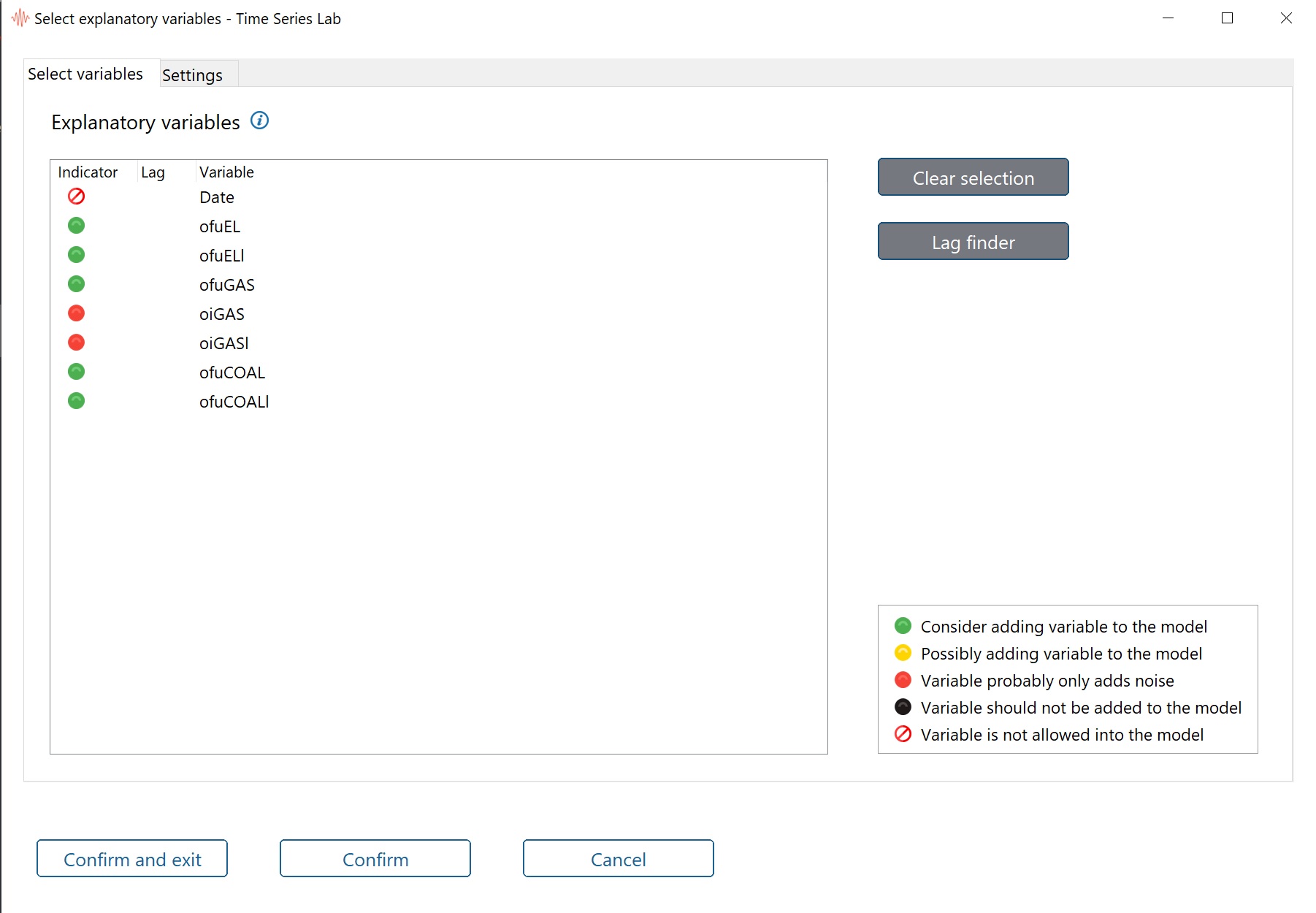
5.1.8.2 Lag finder
5.1.8.3 Settings
5.1.9 Intervention variables
![]() , we see
, we see
EstimationEstimation page of TSL
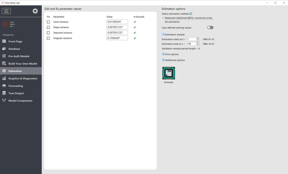
6.1 Edit and fix parameter values
TSL warning for a non-stationary AR(2) process
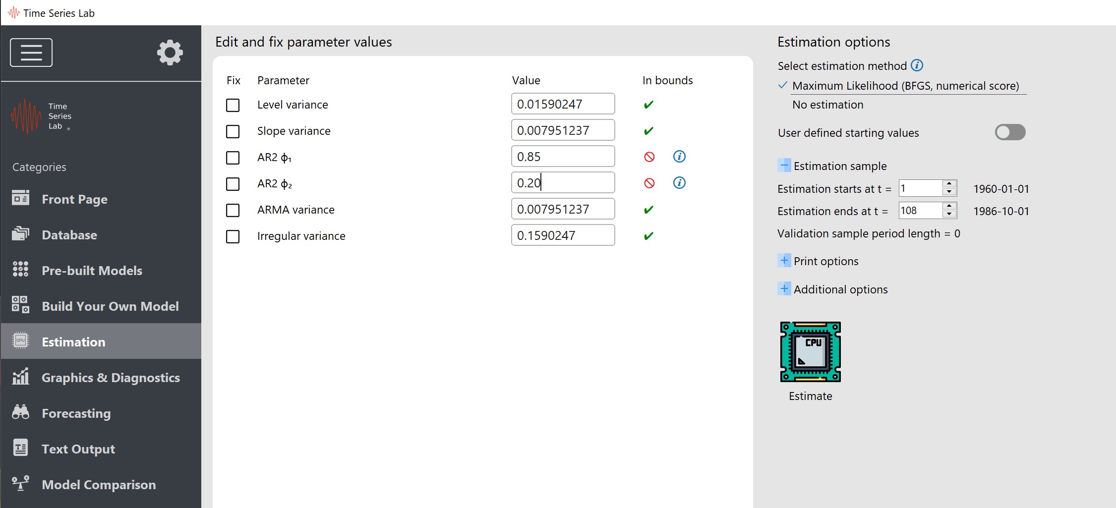
6.2 Estimation options
![]()
Graphical inspection of the estimation results is an important step in the time series modelling
process. You are taken automatically to the Graphics page of TSL after the estimation
process has finished. We can manually reach this page by clicking the button shown
on the left. The default graphical output for the Nile data illustration is displayed in
Figure 7.1.
Graphics and diagnostics7.1 Selecting plot components
Graphical output for Nile data and Local Level model

Autocorrelation plot of Nile data standardized residuals
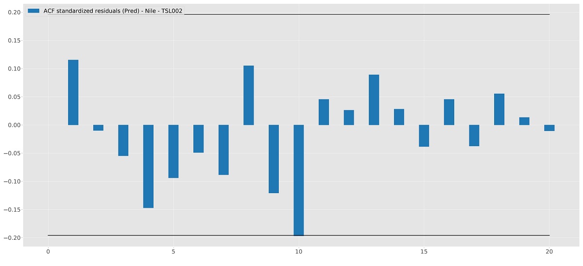
7.2 Plot area
![]()
7.3 Additional options
7.3.1 Plot confidence bounds
Graphical output for Nile data and Local Level model
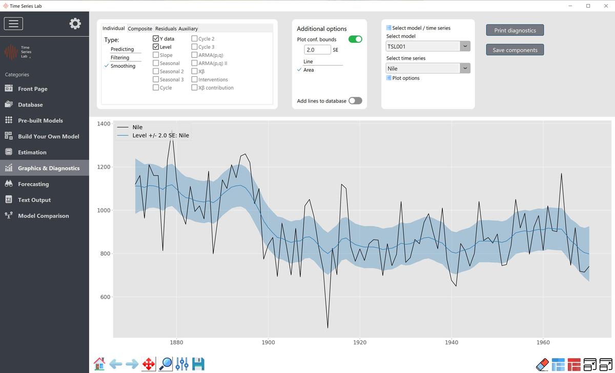
7.3.2 Add lines to database
7.3.3 Select model / time series
7.3.4 Plot options
7.4 Print diagnostics
TSL diagnostics window
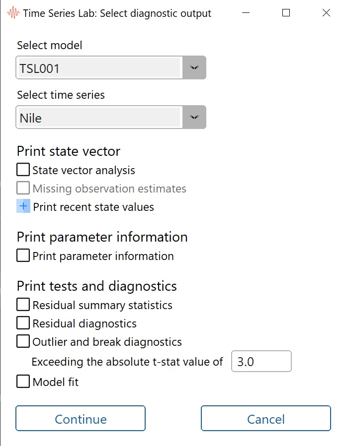
7.4.1 State vector analysis
7.4.2 Missing observation estimates
7.4.3 Print recent state values
7.4.4 Print parameter information
7.4.5 Residual summary statistics
7.4.6 Residual diagnostics
7.4.7 Outlier and break diagnostics
7.4.8 Model fit
7.5 Save components
The Forecasting page of TSL with the Nile data as illustration looks like Figure 8.1. The
Forecasting page can be reached by using the button as shown on the left. Forecasting a time series
is often of great interest for users because being able to say “something” about the future can be of
great value. Forecasts need to be evaluated in some way. This is usually done by loss functions
which we will discuss later in this section. A forecast comparison between different models
and for different forecast horizons can be performed on the Model comparison page, see
Chapter 10.
ForecastingForecasting page of TSL
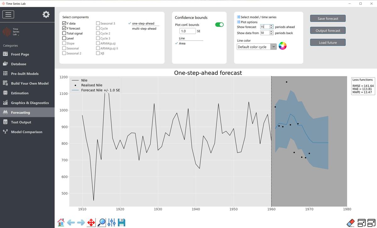
8.1 Forecast components
Multi-step-ahead forecast for Local Level model
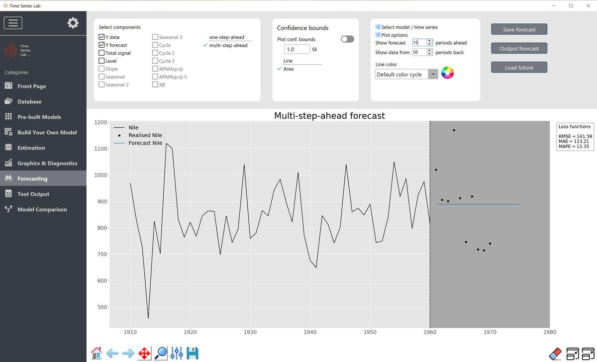
8.2 Additional options
8.2.1 Plot confidence bounds
8.2.2 Select model / time series
8.2.3 Plot options
8.3 Load future
![]()
8.4 Save forecast
8.5 Output forecast
Written output is provided on the Text output page of TSL which can be reached by using
the button as displayed on the left. Written output can be anything from optimization
results, warnings, to output of diagnostic tests. An example of text output printed by TSL
during and after the estimation of the Local Level model and the Nile data is shown in
Figure 9.1.
Text outputText output for the Local Level model
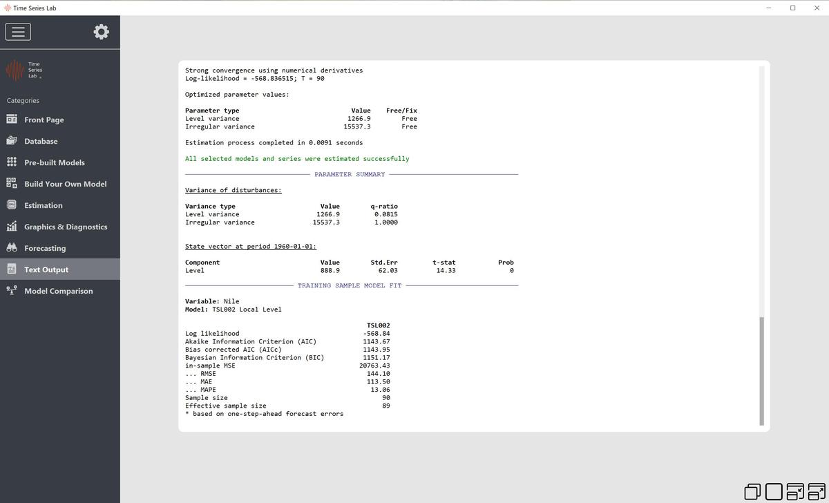
The Model comparison page of TSL can be reached by using the button as displayed on the left. It
is an import page because forecasting performance of different models can be compared with each
other. For each model, the page shows forecast errors up to $h=50$ time periods ahead.
This is useful to see if a model performs well on, for example, shorter or longer forecast
horizons.
Model comparison
![]()
10.1 Loss calculation procedure
10.2 Start loss calculation
The Batch module of TSL is designed to program TSL rather than go through all modelling steps
and menus manually. This way, TSL can be used to automate the modelling and forecasting of time
series. A Batch program needs to be written only once and can then be used each time
again to assign tasks to TSL. It also allows you to schedule TSL, for example to run the
Batch program every morning at 07:00 or to run the Batch program repeatedly every 60
seconds.
Batch module
The easiest way to see all features of the Batch module is to look at some example Batch programs which can be found in the "batch_programs" folder of the installation directory.
Additionally, most of the Case studies have Batch programs that replicate the analysis. Links to the Batch programs can be found at the page of each of the Case studies. For example, here you can download the Batch program for the business cycle Case study (business_cycle.txt).
More details on the Batch module will follow at a later stage.
Batch module with example program
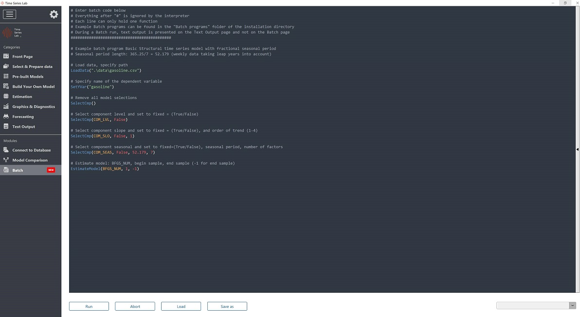
Appendix A
Dynamic modelsNumber of cases of Dengue in a region of Venezuela
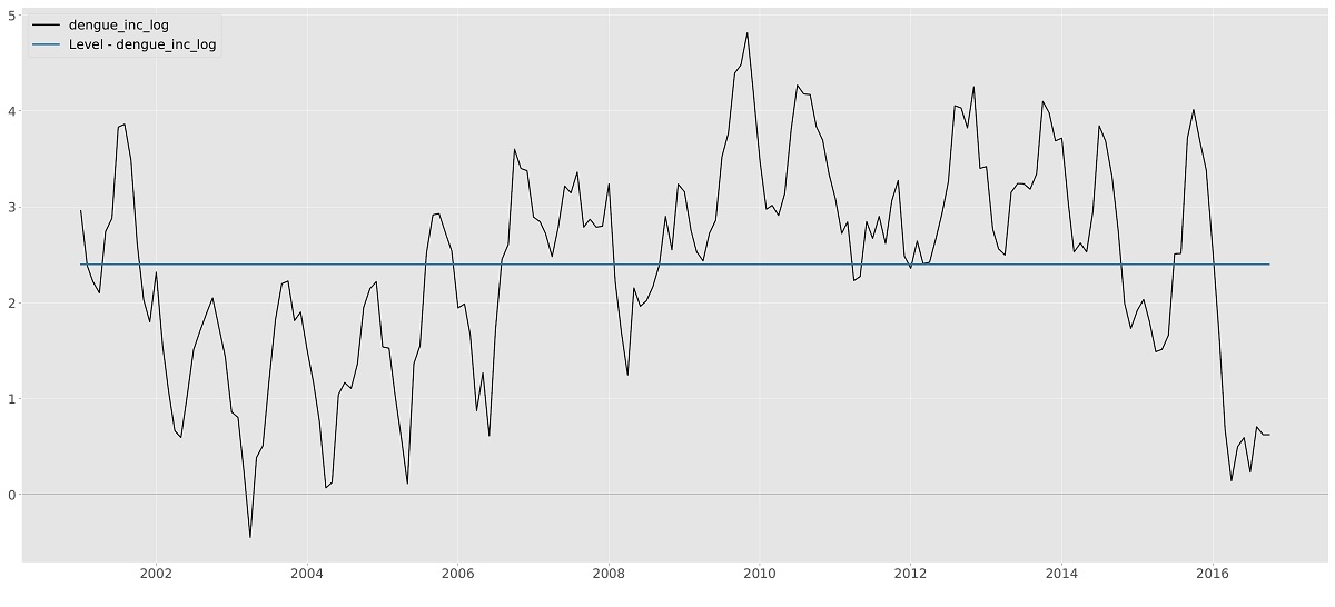
Cases of Dengue and time-varying mean
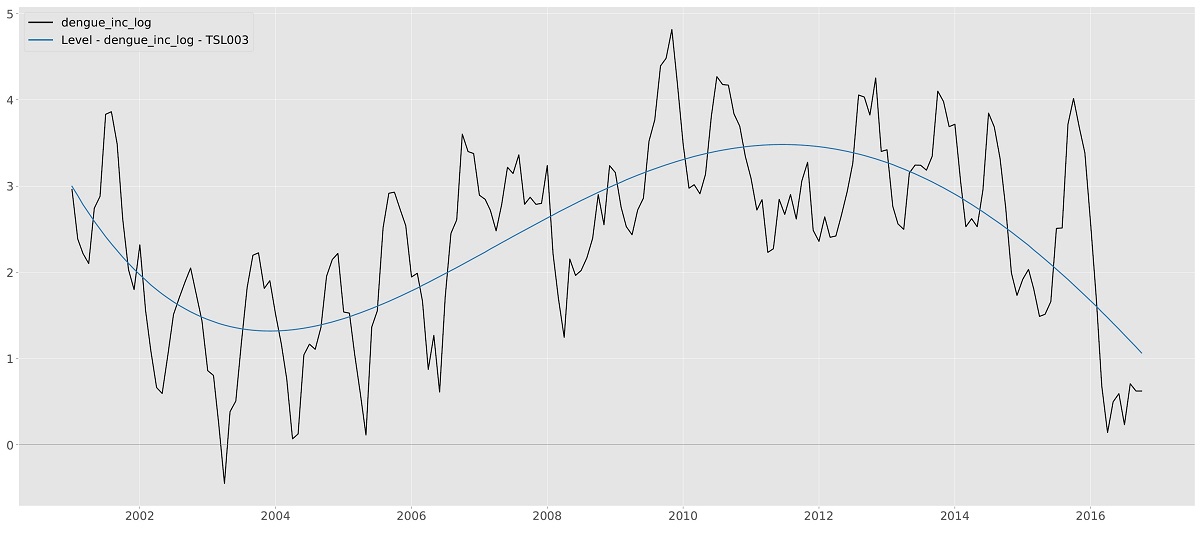
Number of cases of Dengue with dynamic mean with monthly effect
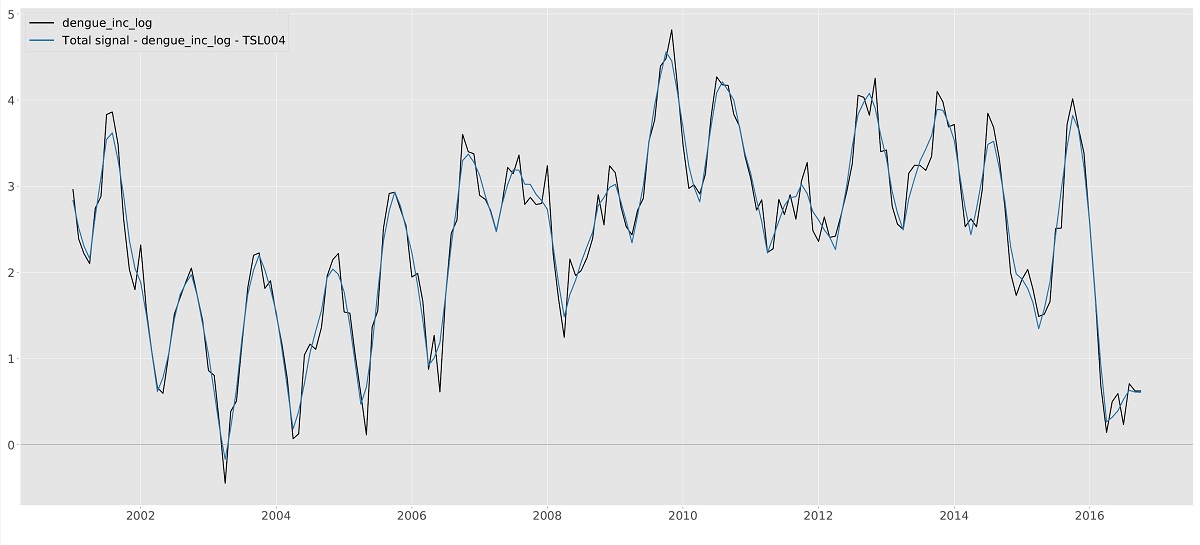
Appendix B
State Space modelsAppendix C
Score-driven modelsAppendix D
Submodels of score-driven modelsD.1 The ARMA model
D.2 The GARCH model
Bibliography